博客内容Blog Content
大语言模型LLM之构建GPT骨架 Building A GPT Framework of Large Language Models (LLMs)
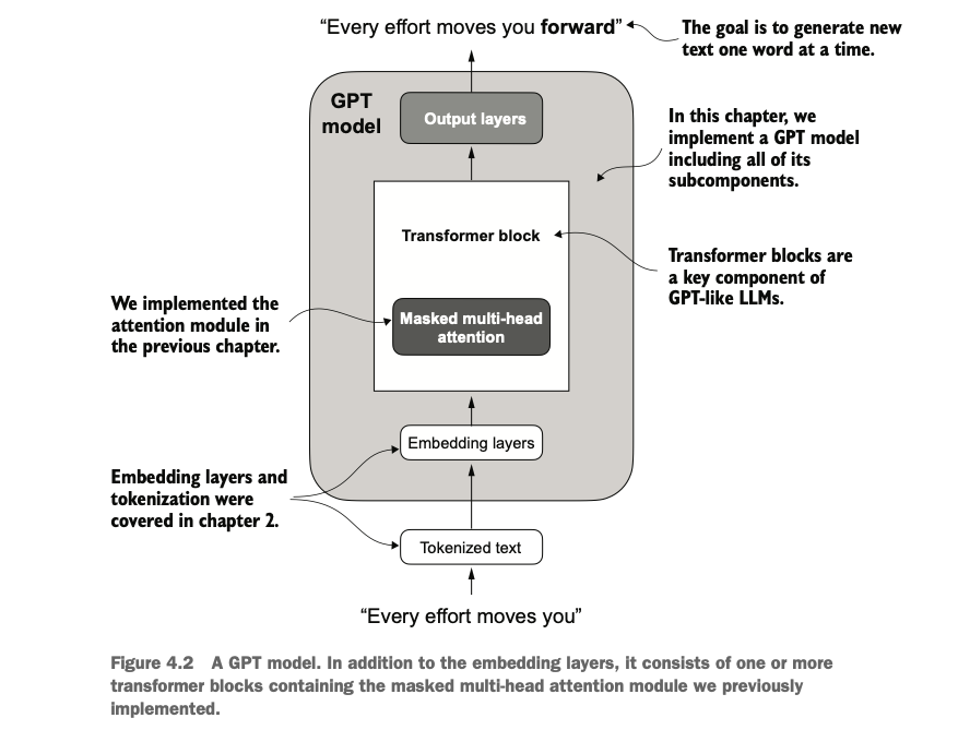
实现一个包含了多头注意力和前馈网络的Transformer块,并将其与token化与logits映射连接起来,实现可预测词功能 Implement a Transformer block that includes multi-head attention and feed-forward networks, and connect it with tokenization and logits mapping to enable word prediction functionality.
4.0 总览 Overview
![]() 4. Implementing a GPT model from scratch to generate text.ipynb
4. Implementing a GPT model from scratch to generate text.ipynb
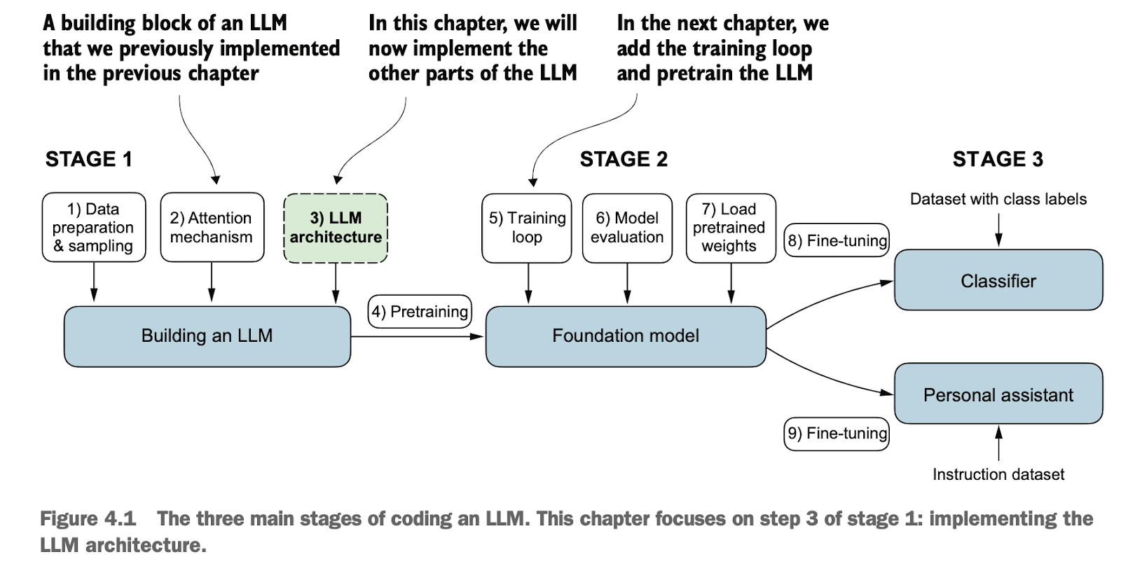
编写类似 GPT 的大语言模型 (LLM),能够训练生成类人文本
对网络层激活进行归一化,以稳定神经网络训练
在深度神经网络中添加快捷连接
实现 Transformer 块以创建各种规模的 GPT 模型
计算 GPT 模型的参数数量和存储需求
Develop a large language model (LLM) similar to GPT, capable of training to generate human-like text.
Normalize activations in network layers to stabilize neural network training.
Add shortcut connections in deep neural networks.
Implement Transformer blocks to create GPT models of various scales.
Calculate the parameter count and storage requirements of GPT models.
4.1 构建GPT骨架 Building the GPT Framework
4.1.1 核心GPT参数集 Core GPT Parameter Set
之前章节以小规模参数作演示为主,现在我们要将模型扩展到一个小型GPT-2模型的规模,具体来说,是最小版本,包含 约1.2 亿参数,在深度学习和 LLM的背景下,术语“参数”指的是模型的可训练权重。这些权重本质上是模型的内部变量,会在训练过程中通过最小化特定的损失函数进行调整和优化。这种优化使模型能够从训练数据中学习。
In previous sections, we primarily demonstrated with small-scale parameters. Now, we aim to scale the model up to the size of a small GPT-2 model. Specifically, this is the smallest version, containing approximately 120 million parameters. In the context of deep learning and LLMs, the term "parameters" refers to the trainable weights of the model. These weights are essentially the internal variables of the model, which are adjusted and optimized during training by minimizing a specific loss function. This optimization allows the model to learn from training data.
神经网络层的参数数量由权重矩阵的维度决定,参数规模的增加会显著提升计算需求。
The number of parameters in a neural network layer is determined by the dimensions of its weight matrices. Increasing the scale of parameters significantly raises computational requirements.
GPT-2 和 GPT-3 的架构相似,但 GPT-3 的参数数量(1750 亿)远超 GPT-2(1.5 亿到 15 亿),并使用了更多的训练数据。由于 GPT-2 的预训练权重公开且硬件需求较低(可在笔记本电脑上运行),它更适合学习和实验,而 GPT-3 的训练和推理需要高性能 GPU 集群,计算成本极高,例如使用 V100 GPU 训练需 355 年。
The architectures of GPT-2 and GPT-3 are similar, but GPT-3 has far more parameters (175 billion) compared to GPT-2 (ranging from 150 million to 1.5 billion) and uses more training data. Since GPT-2's pre-trained weights are publicly available and its hardware requirements are relatively low (it can be run on a laptop), it is more suitable for learning and experimentation. On the other hand, training and inference with GPT-3 require high-performance GPU clusters and incur extremely high computational costs. For example, training GPT-3 on V100 GPUs would take 355 years.
我们的GPT模型参数配置如下
Our GPT model's parameter configuration is as follows:
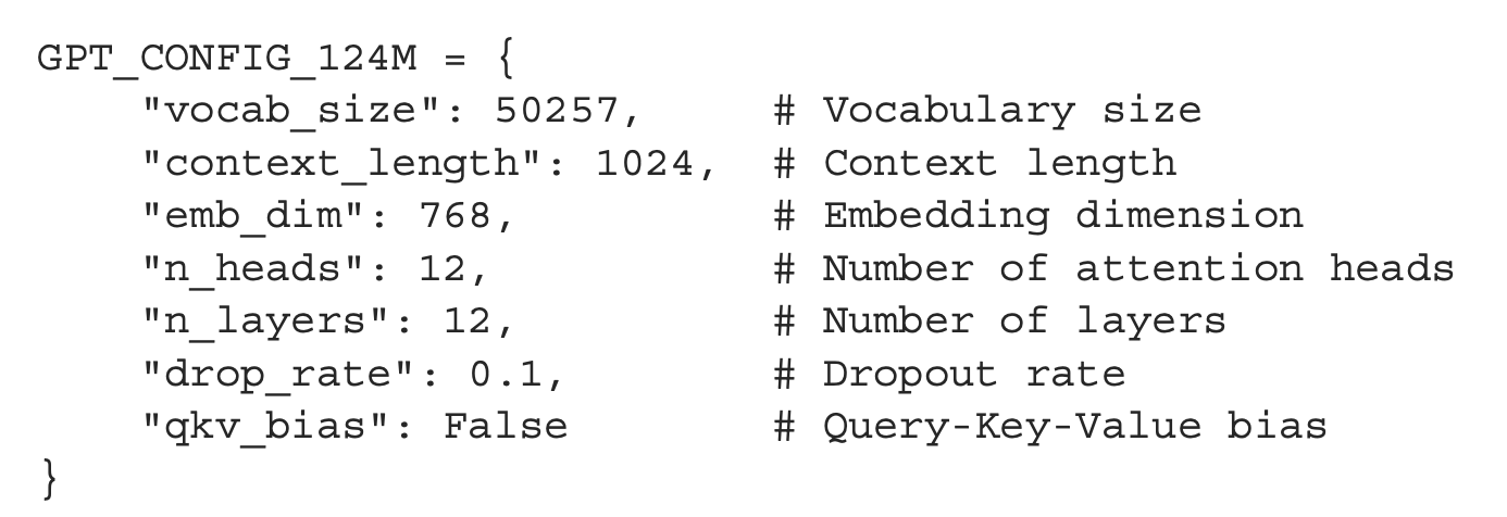
vocab_size:表示词汇表的大小,为 50,257 个单词,由 BPE 分词器使用。
context_length:表示模型可处理的输入 token 的最大数量,通过位置嵌入控制。
emb_dim:表示嵌入维度,将每个 token 转换为一个 768 维的向量。
n_heads:表示多头注意力机制中的注意力头的数量。
n_layers:表示模型中 Transformer 块的数量(将在后续讨论中介绍)。
drop_rate:表示丢弃机制的强度,数值为 0.1 时表示随机丢弃 10% 的隐藏单元,以防止过拟合。
qkv_bias:决定是否在多头注意力机制中的查询、键和值的计算中包含偏置向量。
vocab_size: Represents the size of the vocabulary, which contains 50,257 words and is used by the BPE tokenizer.
context_length: Represents the maximum number of input tokens the model can process, controlled via positional embeddings.
emb_dim: Represents the embedding dimension, which converts each token into a 768-dimensional vector.
n_heads: Represents the number of attention heads in the multi-head attention mechanism.
n_layers: Represents the number of Transformer blocks in the model (to be discussed later).
drop_rate: Represents the dropout rate, with a value of 0.1 indicating that 10% of the hidden units are randomly dropped to prevent overfitting.
qkv_bias: Determines whether bias vectors are included in the computation of queries, keys, and values in the multi-head attention mechanism.
4.1.2 实现GPT的骨架 Implementing the GPT Framework
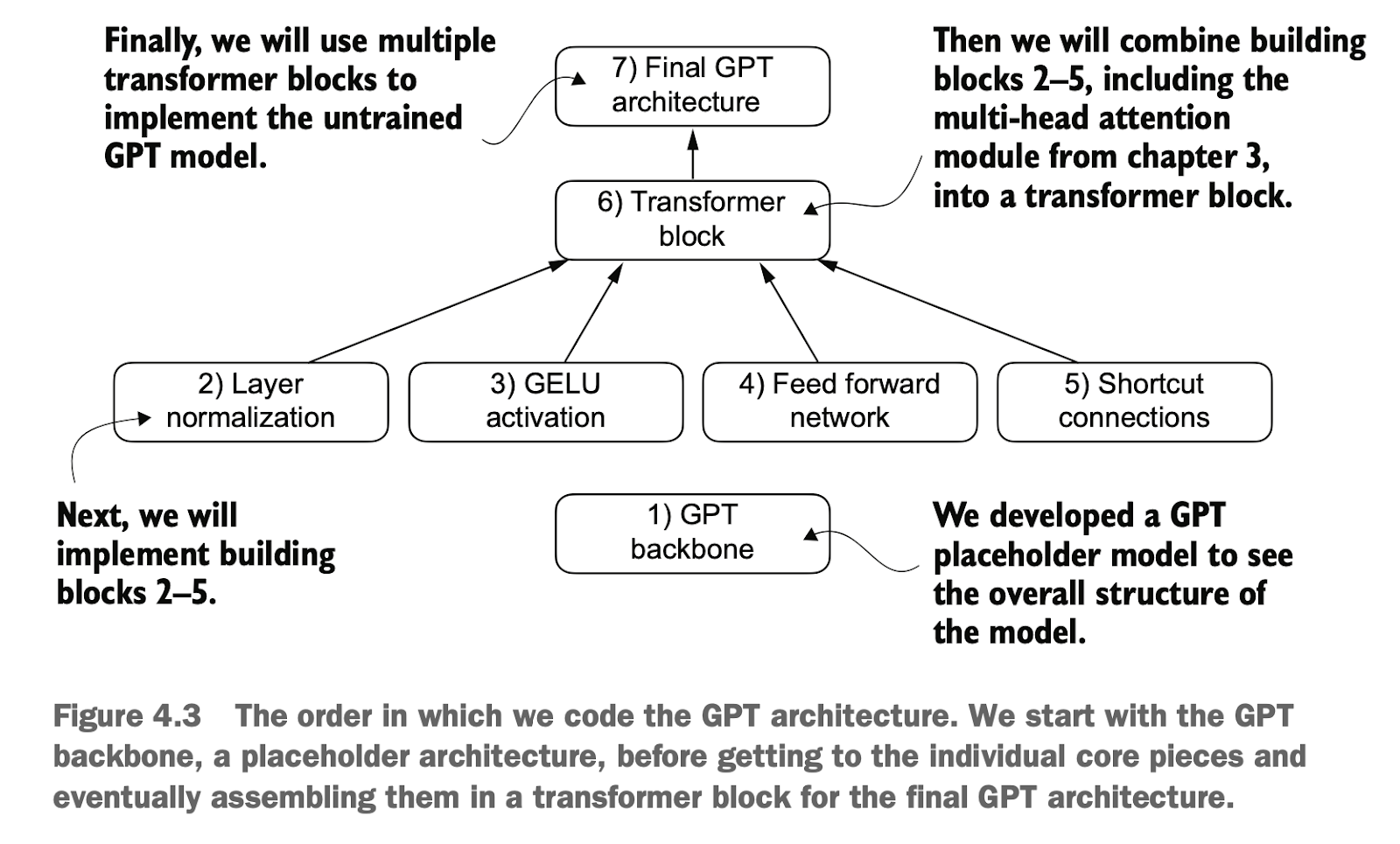
使用该配置,我们将实现一个 GPT 占位架构(DummyGPTModel)。用于提供一个骨架的整体视图,说明各部分如何结合在一起,以及需要实现哪些其他组件来组装完整的 GPT 模型架构。
Using this configuration, we will implement a placeholder GPT architecture (DummyGPTModel) to provide an overall skeleton view of how the components fit together and identify the additional components required to assemble a complete GPT model architecture.
这段代码实现了一个简化版的 GPT 模型,用于演示 GPT 模型的基本结构
This code implements a simplified version of a GPT model to demonstrate the basic structure of a GPT model.
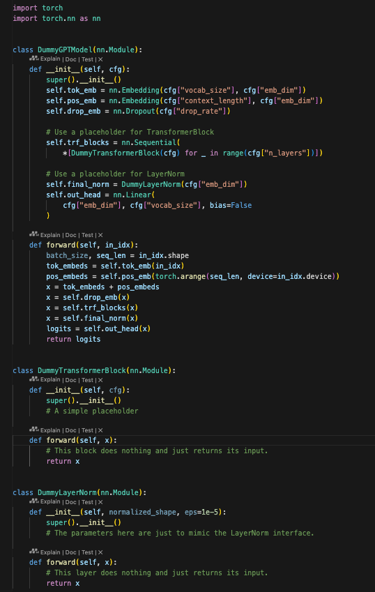
输入:一个词索引张量(如 [6109, 3626, 6100, 345])。
处理流程:
将词索引映射到词嵌入(tok_emb)。
加上位置嵌入(pos_emb)。
经过 Dropout 随机丢弃部分嵌入值。
通过多层 Transformer 块(这里是占位符,先不做任何处理,后续优化)。
归一化到embedding维度预测概率(占位符,先不做任何处理,后续优化)。
该embedding预测投影到词汇表,生成 logits。
输出:
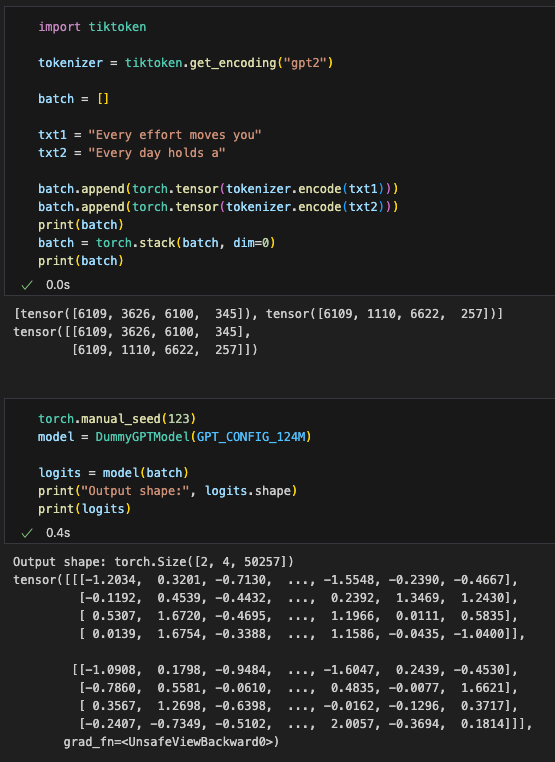
每个时间步的 logits,表示预测下一个可能词对应50257个词汇的概率分布。
模型输出 logits,用于预测下一个词的分布,例如输入是完整的句子,输出可以被理解为 txt1 和 txt2 的第 2 到第 5 个词的预测分布(实际上是第 1 到第 4 个词的偏移后向下一个词的预测分布),损失函数会用于比较预测的分布和目标词的实际索引。
输出是logits是为了灵活性,下游可用softmax处理用于预测词,也可以作其它处理如分类
Input: A tensor of word indices (e.g., [6109, 3626, 6100, 345]).
Processing Flow:
Map the word indices to word embeddings (tok_emb).
Add positional embeddings (pos_emb).
Apply dropout to randomly discard part of the embedding values.
Pass through multiple Transformer blocks (currently placeholders with no processing; will be optimized later).
Normalize to the embedding dimension to predict probabilities (currently a placeholder, to be optimized later).
Project the embeddings onto the vocabulary to generate logits.
Output:
The logits for each time step, representing the probability distribution of the next possible word over the 50,257-word vocabulary.
The model outputs logits, which are used to predict the distribution of the next word. For example, if the input is a complete sentence, the output can be understood as the predicted distributions for the 2nd to 5th words in txt1 and txt2(in practice, it predicts the next word for the 1st to 4th words with an offset). A loss function is used to compare the predicted distribution with the actual indices of the target words.
The output is provided as logits for flexibility. Downstream tasks can apply a softmax function for word prediction or use the logits for other tasks, such as classification.
4.2 实现层归一化 Implementing Layer Normalization
4.2.1 层归一化概念 The Concept of Layer Normalization
接下来,为了解决梯度消失或梯度爆炸问题,我们将实现层归一化(Layer Normalization),以提高神经网络训练的稳定性和效率。这里先介绍一下层归一化的基本概念。
Next, to address the problem of vanishing or exploding gradients, we will implement Layer Normalization to improve the stability and efficiency of neural network training. Let’s first introduce the basic concept of layer normalization.
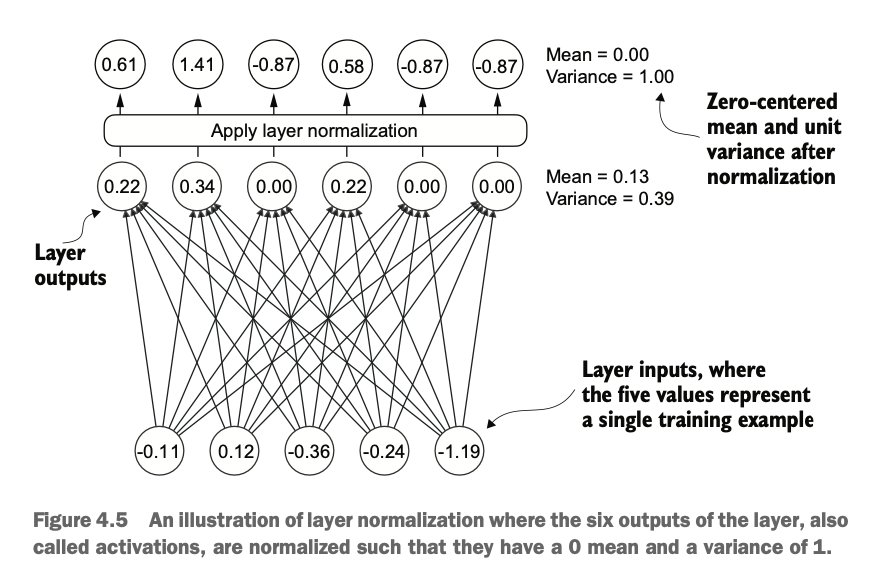
层归一化相当于一种标准化的方法,主要目的是调整神经网络层的激活值输出,使其均值为 0,方差为 1(即单位方差)。这种调整可以加速权重的收敛,并确保训练过程的一致性和可靠性。
Layer normalization is a type of normalization technique designed to adjust the activation outputs of neural network layers so that they have a mean of 0 and a variance of 1 (unit variance). This adjustment accelerates the convergence of weights and ensures consistency and reliability during the training process.
如图,激活层将每层输出的数据处理,归一化到均值为0,方差为1
As illustrated, the activation layer processes each layer’s output data, normalizing it to have a mean of 0 and a variance of 1.
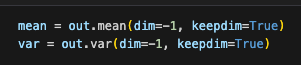
使用mean和var计算均值和方差,dim指定按哪个方向进行“压扁”聚合,或者沿着哪个维度消掉它(压扁后该方向维度应该要会消失,但是可以用keepdim=True保留着,dim=-1表示按最后一个维度,如二维是把”列-行“中的行压扁,三维是把”高-列-行“的行压扁)
The computation of normalization involves using mean and var to calculate the mean and variance, where dim specifies along which dimension the aggregation (or "flattening") happens. After flattening, the target dimension "disappears," but it can be retained using keepdim=True. For example:dim=-1 means normalization is performed along the last dimension.In 2D tensors, it flattens the "row" in the "column-row" structure.In 3D tensors, it flattens the "row" in the "height-column-row" structure.
4.2.2 实现GPT的层归一化 Implementing Layer Normalization in GPT
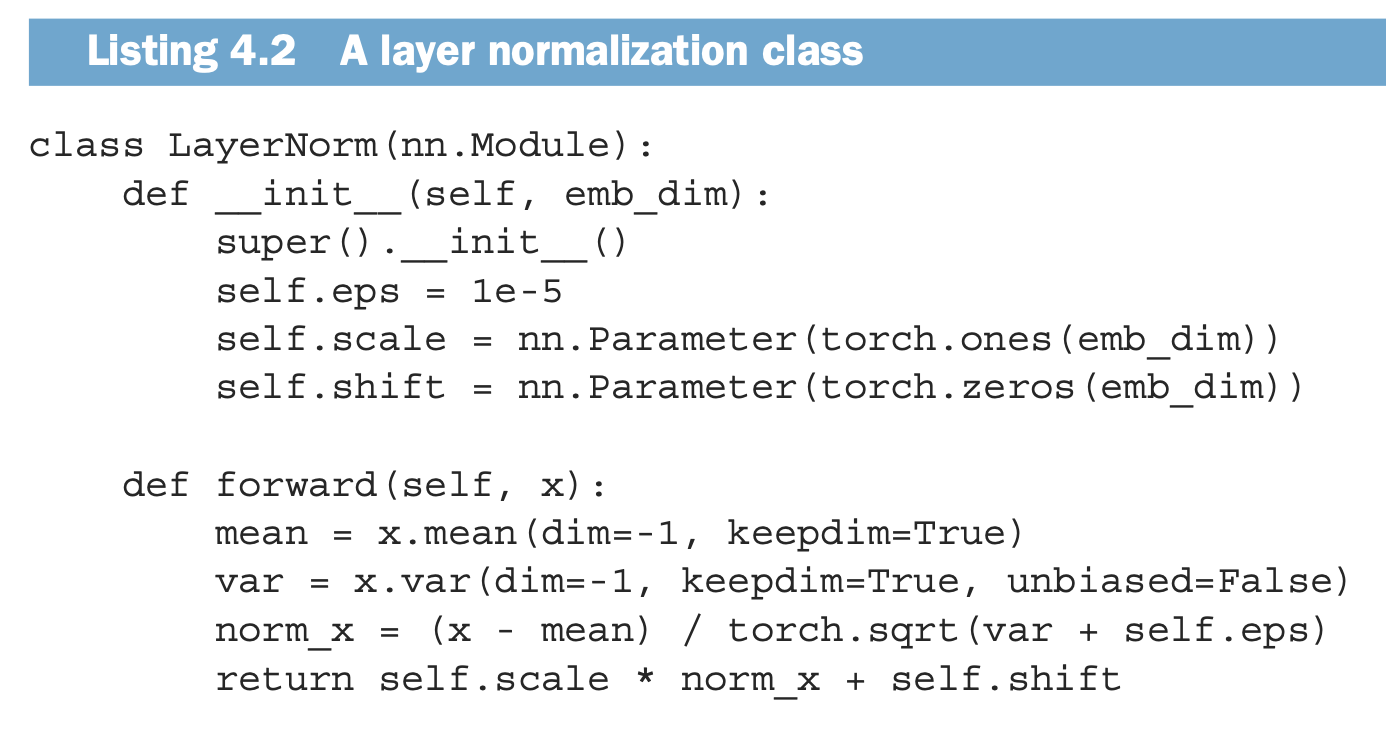
我们接下来使用代码实现了一个自定义的 Layer Normalization(层归一化) 类。Layer Normalization 是一种正则化技术,在这个GPT里归一化层的作用是相当于把经过多层变化的矩阵,映射到emb_dim长度向量即单词维度的空间里,同时解决层过多导致的不稳定问题,
eps: 一个小的常数(epsilon),用于防止除以零的情况(数值稳定性)。
scale 和 shift:学习的缩放和偏移参数,使特征分布能更好够适应当前任务。
返回给foward的内容:经过归一化(标准化 + 缩放 + 偏移)的输入张量。用于后续网络层使用
We will now implement a custom Layer Normalization class in code. Layer normalization is a regularization technique, and in GPT, its purpose is to map matrices transformed through multiple layers into the word-dimensional space (of size emb_dim). It also addresses stability issues caused by too many layers.
eps: A small constant (epsilon) used to prevent division by zero (for numerical stability).scaleandshift: Learnable scaling and shifting parameters that allow the feature distribution to adapt better to the current task.Return value in
forward: The input tensor normalized (standardized + scaled + shifted) and passed to subsequent network layers.
此外,在机器学习中,除了层归一化(Layer Normalization),还有批归一化(Batch Normalization),区别是层归一化沿着最后一个维度(即特征维度),不依赖批量大小;而批归一化沿 batch 和其他维度归一化,依赖批量大小
Additionally, in machine learning, apart from Layer Normalization, there is also Batch Normalization. The key difference is: Layer Normalization performs normalization along the last dimension (i.e., the feature dimension) and does not depend on batch size.Batch Normalization normalizes across the batch and other dimensions, making it dependent on batch size.
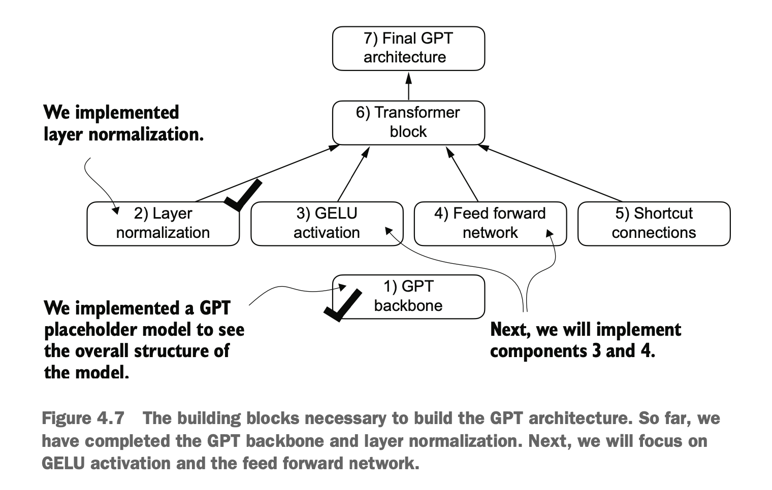
目前为止,我们已实现了第1步的骨架搭建,以及第2步的层归一化的实现,接下来学习前馈网络的GELU激活函数相关概念和代码实现,并在feedforward模块中使用
So far, we have completed Step 1 (building the GPT skeleton) and Step 2 (implementing layer normalization). Next, we will explore the concept and implementation of the GELU activation function, which will be used in the feedforward module.
4.3 实现Transformer层带有激活函数的前馈网络 Implementing Transformer Feedforward Networks with Activation Functions
4.3.1 激活函数概念 Concept of Activation Functions
激活函数是神经网络中的一个关键组件,其主要任务是引入非线性,以便神经网络能够学习和表示复杂的非线性关系。没有激活函数的网络(仅包含线性变换)只能表示线性关系,而无法处理更复杂的问题。
Activation functions are a critical component of neural networks. Their primary task is to introduce non-linearity, enabling neural networks to learn and represent complex non-linear relationships. Without activation functions, networks (which consist only of linear transformations) can only represent linear relationships, rendering them incapable of handling more complex problems.
历史上,ReLU 激活函数因其简单性和在各种神经网络架构中的有效性而被广泛使用。然而,在 LLM 中,除了传统的 ReLU,还采用了其他几种激活函数。其中两个著名的例子是 GELU(高斯误差线性单元)和 SwiGLU(Swish 门控线性单元)。GELU 和 SwiGLU 是更复杂且平滑的激活函数,分别结合了高斯分布和 sigmoid 门控线性单元的特性。与更简单的 ReLU 不同,它们为深度学习模型提供了更好的性能。
Historically, the ReLU activation function has been widely used due to its simplicity and effectiveness in various neural network architectures. However, in LLMs (Large Language Models), several other activation functions are employed in addition to traditional ReLU. Two well-known examples are GELU (Gaussian Error Linear Unit) and SwiGLU (Swish Gated Linear Unit). GELU and SwiGLU are more complex and smoother activation functions, combining the characteristics of Gaussian distributions and sigmoid-based gated linear units, respectively. Unlike the simpler ReLU, they provide better performance for deep learning models.
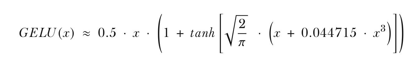
GELU 激活函数可以通过多种方式实现,其精确形式定义为: GELU(x) = x⋅Φ(x),其中 Φ(x) 是标准高斯分布的累积分布函数(CDF)。 然而,在实际应用中,通常会实现一种计算成本更低的近似版本(原始 GPT-2 模型也使用了这种通过曲线拟合找到的近似版本)。
The GELU activation function can be implemented in multiple ways, with its exact form defined as: GELU(x) = x ⋅ Φ(x), where Φ(x) is the cumulative distribution function (CDF) of the standard Gaussian distribution. However, in practice, a computationally cheaper approximate version is often implemented (for instance, the original GPT-2 model uses such an approximation based on curve fitting).
比较GELU和ReLU的图可发现
Comparing GELU and ReLU
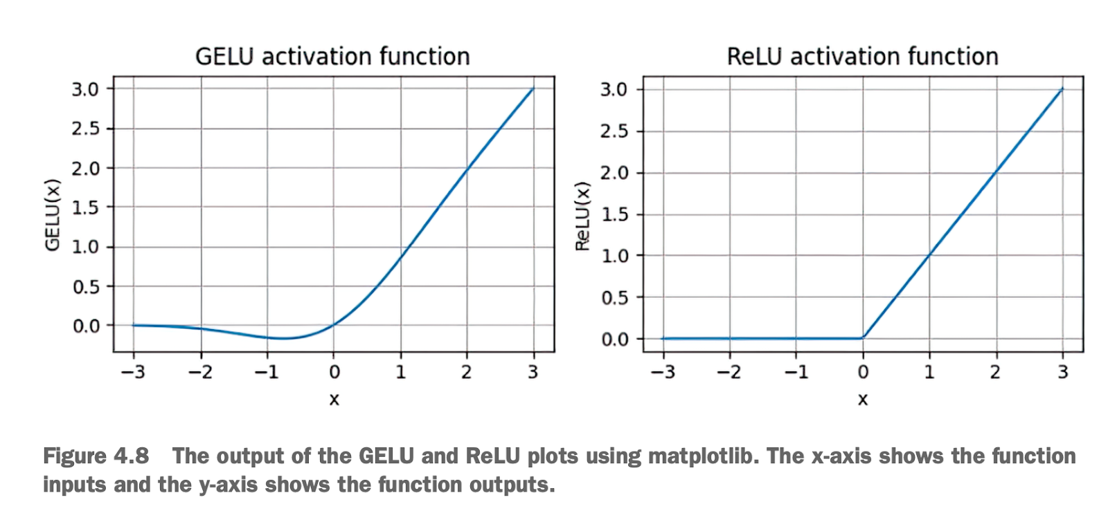
ReLU 是一种简单、高效的激活函数,但其对负值输入的输出为零,可能导致神经元“死亡”,且在 x = 0 处的尖锐拐角可能阻碍优化。
GELU 是一种平滑的激活函数,能更自然地处理负值输入,保持非零梯度,避免神经元“死亡”,并允许对参数进行更细致的调整。
在现代深度学习模型(如 Transformer 和 LLM 中),GELU 更适合作为激活函数,因为它能更好地支持复杂网络的优化和性能提升。
ReLU is a simple and efficient activation function. However, it outputs zero for negative input values, which may result in "dead neurons" in the network. Additionally, the sharp corner at x = 0 could obstruct optimization.
GELU is a smoother activation function that can naturally handle negative inputs, maintain non-zero gradients, and avoid "dead neurons." It also allows for more precise parameter adjustments.
In modern deep learning models (such as Transformers and LLMs), GELU is better suited as an activation function because it supports the optimization and performance enhancement of complex networks more effectively.
4.3.2 实现带GELU激活函数前馈网络模块 Implementing a Feedforward Network Module with GELU Activation Function
在 LLM(如 GPT)中的前馈网络实现中,我们将实现一个小型神经网络子模块,它是 LLM(大型语言模型)中 Transformer 块的一部分。
In the feedforward network implementation of LLMs (e.g., GPT), we will implement a small neural network submodule, which is a part of the Transformer block in LLMs.
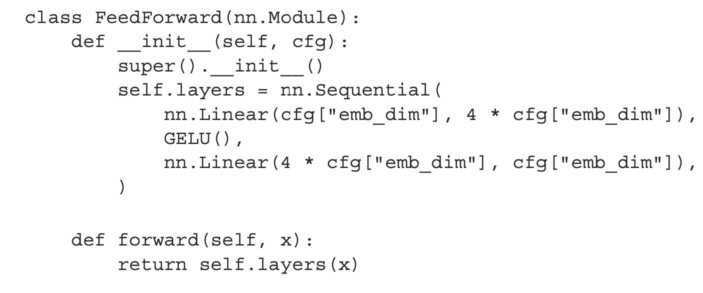
具体而言,我们将实现一个前馈神经网络模块(FeedForward)的例子,并使用 GELU 激活函数 来增强网络的性能,其由以下部分组成:
两个线性层(nn.Linear):
第一个线性层将输入维度(emb_dim)扩展 4 倍。
第二个线性层将维度缩回到原始的 emb_dim。
GELU 激活函数(GELU()):
插入在两个线性层之间,增加非线性能力。
Specifically, we will implement an example of a feedforward neural network module (FeedForward) and use the GELU activation function to enhance the network's performance. This module consists of the following components:
Two Linear Layers (nn.Linear):
The first linear layer expands the input dimension (emb_dim) by 4 times.
The second linear layer reduces the dimension back to the original emb_dim.
GELU Activation Function (GELU()):
Inserted between the two linear layers to increase non-linear capabilities.
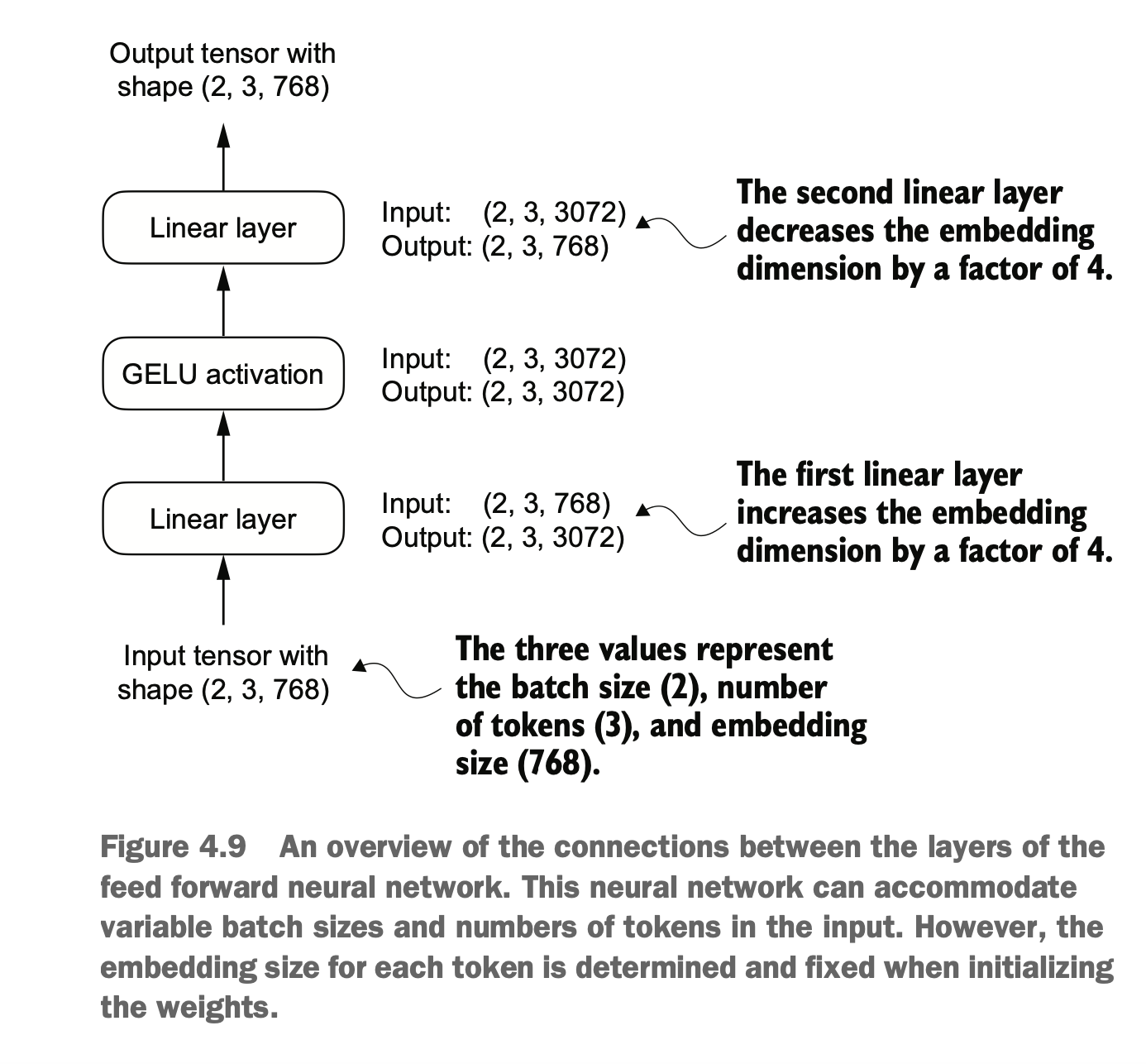
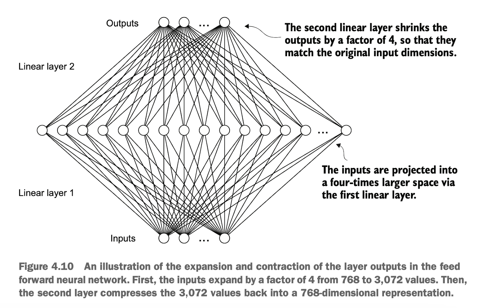
这里的FeedForward 模块在提升模型从数据中学习和泛化能力方面起着至关重要的作用。虽然该模块的输入和输出维度保持一致,但它内部通过第一个线性层将嵌入维度扩展到更高维空间(如图 4.10 所示)。这一扩展随后经过一个非线性的 GELU 激活函数处理,再通过第二个线性变换将维度收缩回原始大小。这样的设计允许模型探索更加丰富的表示空间。
The FeedForward module plays a crucial role in improving the model's ability to learn and generalize from data. Although the input and output dimensions of this module remain consistent, it internally expands the embedding dimension to a higher-dimensional space through the first linear layer (as shown in Figure 4.10). This expansion is then processed by a non-linear GELU activation function, followed by a second linear transformation to reduce the dimension back to its original size. This design allows the model to explore a richer representation space.
这种“扩展-收缩”机制,不仅提高了模型的特征学习能力,还保持了架构的计算效率和参数规模。
This "expand-reduce" mechanism not only enhances the model's feature learning capability but also maintains computational efficiency and parameter scalability.
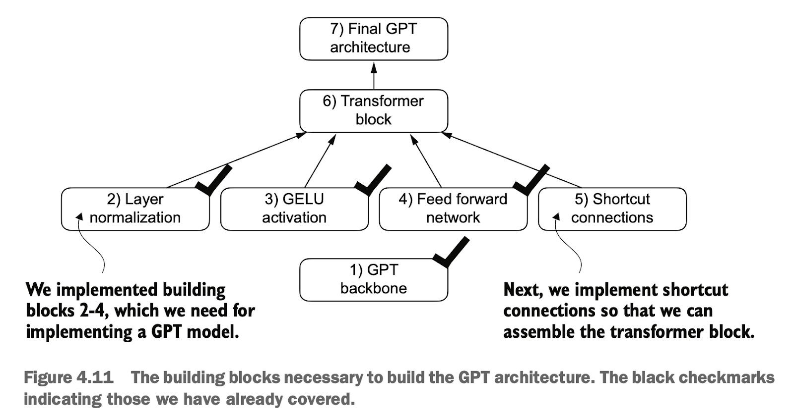
目前为止,我们已实现了第1步的骨架搭建,以及第2步的层归一化的实现,以及第3步带GELU激活函数的前馈网络相关概念和代码实现,接下来我们要学习我们将讨论在神经网络的不同层之间插入 快捷连接(shortcut connections) 的概念和代码实现
So far, we have implemented step 1, the skeleton construction of the module, step 2, the implementation of layer normalization, and step 3, the related concepts and code implementation of the feedforward network with the GELU activation
4.4 实现Transformer层快捷连接 Implementing Shortcut Connections in Transformer Layers
快捷连接(shortcut connections),也称为跳跃连接(skip connections)或残差连接(residual connections)。
Shortcut connections, also known as skip connections or residual connections, are a fundamental concept in deep learning.
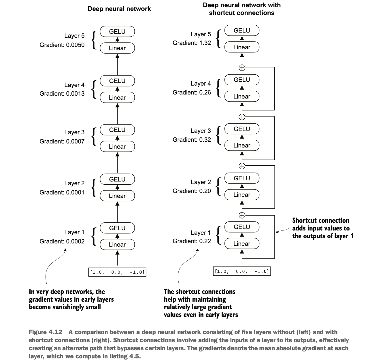
梯度消失问题是指在训练过程中,梯度(用于指导权重更新的量)在反向传播过程中逐渐变小,从而难以有效训练较早的网络层。因此快捷连接是在计算机视觉中的深层网络(尤其是残差网络)中提出的,目的是缓解梯度消失问题。
The vanishing gradient problem refers to the phenomenon where gradients (used to guide weight updates) become progressively smaller during backpropagation, making it challenging to effectively train earlier layers of a network. Shortcut connections were introduced in deep networks for computer vision, particularly in residual networks (ResNets), to alleviate the vanishing gradient problem.
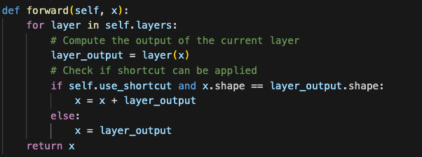
下图显示了快捷连接通过跳过一个或多个层,创建了一条供梯度在网络中流动的替代、较短路径。这是通过将某一层的输出与后续层的输出相加来实现的。这也是为什么这些连接被称为跳跃连接的原因。在训练的反向传播过程中,它们在保持梯度流动方面起到了至关重要的作用。
The diagram below shows how shortcut connections create an alternative, shorter path for gradients to flow through the network by skipping one or more layers. This is achieved by adding the output of a certain layer to the output of subsequent layers. This is why these connections are also called skip connections. During backpropagation, they play a crucial role in maintaining the flow of gradients.
从图中可以看到,DNN在方向传播后回到layer0时梯度变得越来越小,而加了快捷链接的DNN在回到layer0时仍然保持梯度的稳定
The diagram illustrates that in a DNN, gradients become progressively smaller when flowing back to layer 0 during backpropagation. However, with shortcut connections, the gradients remain stable even when they reach layer 0.
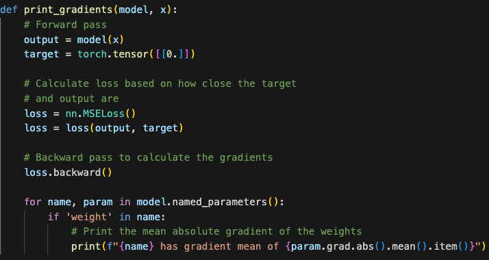
在python中,可通计算output和target的损失,并通过backward获取对应梯度
In Python, this functionality can be implemented by computing the loss between the network's output and the target and then using backward propagation to calculate the corresponding gradients.
4.5 在Transformer层连接多头注意力和前馈网络 Connecting Multi-Head Attention and Feedforward Network in the Transformer Layer
简单来说,Transformer 是一种用于处理序列数据的深度学习架构,它的主要任务是学习序列中的模式和关系,并对输入数据进行有效的表示和变换。它的核心特点在于通过自注意力机制和前馈网络,能够高效地捕捉序列中元素之间的关系,同时对每个元素进行独立的处理。
Simply put, a Transformer is a deep learning architecture designed to process sequential data. Its primary goal is to learn patterns and relationships within sequences and effectively represent and transform input data. The key feature of Transformers lies in their ability to efficiently capture relationships between elements in a sequence through self-attention mechanisms and feedforward networks, while processing each element independently.
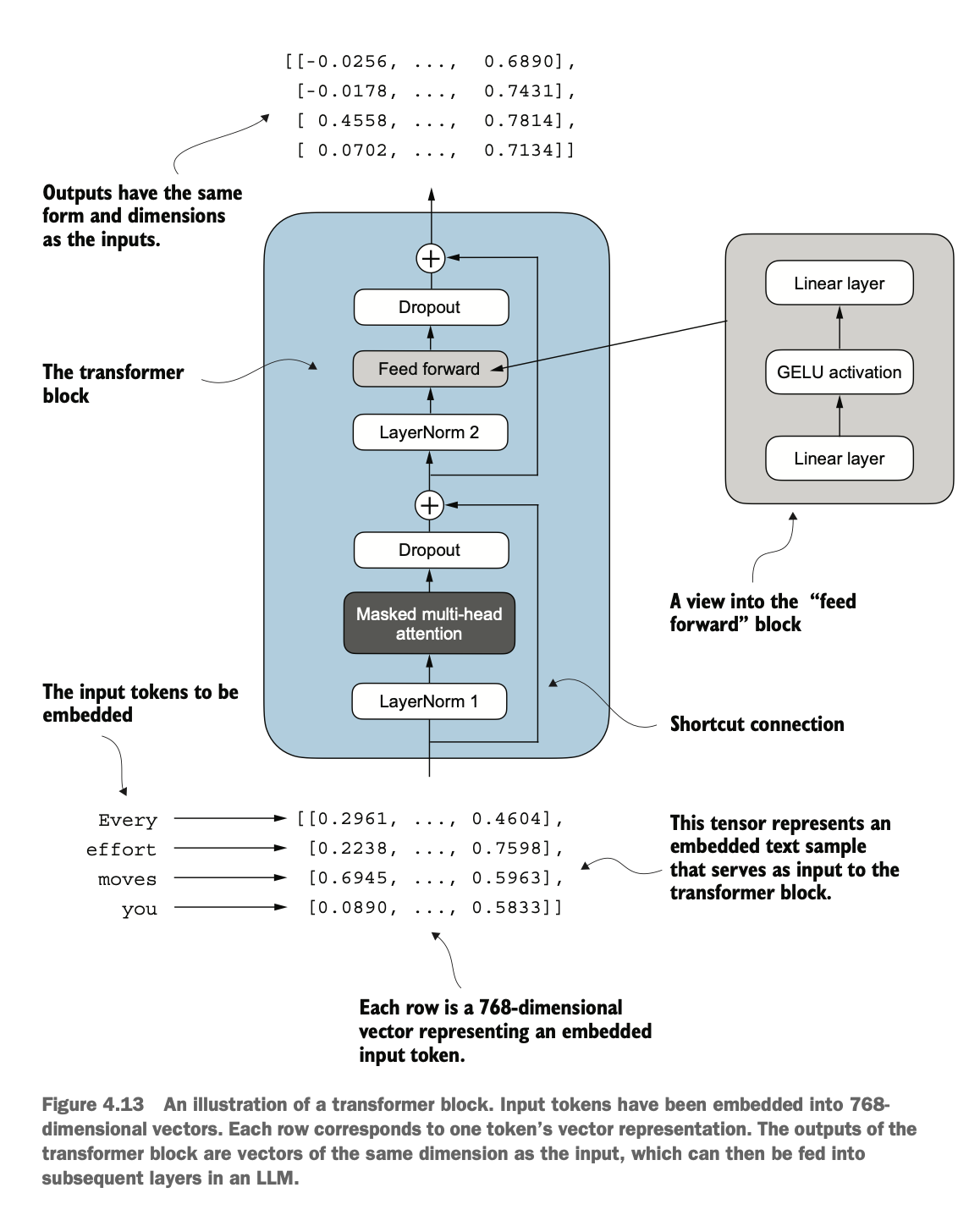
现在,让我们结合我们之前介绍的多个概念,从而实现 Transformer 。下图为一个Transformer的操作,每个元素被固定为维度固定的向量,Transformer 块中的操作(包括多头注意力机制和前馈层)被设计为以一种能够保留维度的方式来变换这些向量,该模块化设计使 Transformer 块可以堆叠多层,逐渐学习更加复杂的模式和关系。
Now, let us combine the various concepts we introduced earlier to implement a Transformer. The diagram shows the operations within a Transformer block, where each element is fixed as a vector of a consistent dimension. The operations in the Transformer block (including multi-head attention mechanisms and feedforward layers) are designed to transform these vectors in a way that preserves their dimensions. This modular design allows Transformer blocks to be stacked in multiple layers, gradually learning more complex patterns and relationships.
Transformer 块是一个 输入-输出维度一致的模块
多头注意力 负责捕捉序列中 token 之间的关系。
前馈网络 负责对每个 token 的表示进行独立的非线性变换。
残差连接、归一化和 Dropout 提升了模型的稳定性和泛化能力。
A Transformer block is a module with identical input and output dimensions.
Multi-head attention is responsible for capturing relationships between tokens in a sequence.
The feedforward network is responsible for performing independent nonlinear transformations on the representation of each token.
Residual connections, normalization, and dropout enhance the stability and generalization ability of the model.
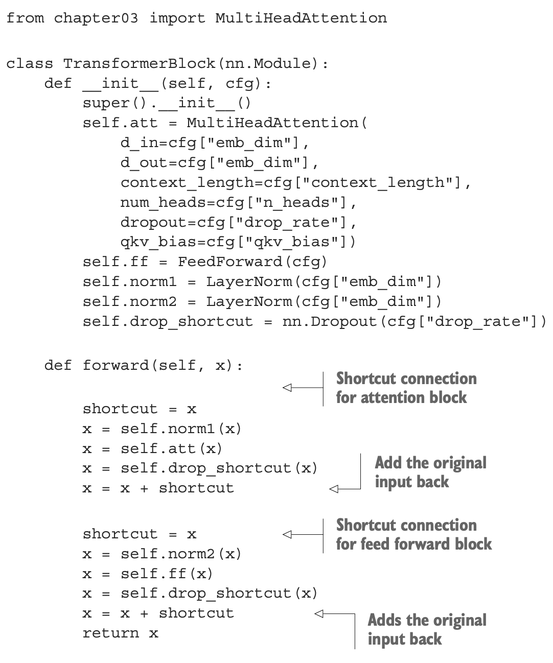
注意,这里Shortcut(残差连接) 虽然跳过了多头注意力机制,然而,它并不会导致信息泄露,主要原因在于多头注意力机制和残差连接的作用是互补的:即使 Shortcut 直接传递了原始输入,后续的前馈网络仍会对叠加后的结果进行进一步处理,因此不会导致模型依赖未屏蔽的未来 token。换句话说,注意力机制在训练时并没有被绕过,残差连接是在它之后加上输入,而不是绕过它或不训练它。
Note that although the shortcut (residual connection) skips the multi-head attention mechanism, it does not lead to information leakage. This is mainly because the roles of the multi-head attention mechanism and residual connection are complementary. Even if the shortcut directly passes the original input, the subsequent feedforward network will further process the combined result. Therefore, the model will not rely on unmasked future tokens. In other words, the attention mechanism is not bypassed during training. The residual connection adds the input after the attention mechanism, rather than skipping it or excluding it from training.
Transformer 是一个深度网络,堆叠了多个 Transformer 块。如果没有 Shortcut,模型需要每一层都学会如何完全重建输入信息,这会让优化过程变得更加困难。而 Shortcut 允许模型只专注于学习输入信息的“增量变化”。
The Transformer is a deep network composed of multiple stacked Transformer blocks. Without shortcuts, the model would need each layer to completely reconstruct the input information, making the optimization process more difficult. Shortcuts allow the model to focus only on learning the "incremental changes" in the input information.
Transformer 块在处理数据序列时会保留输入和输出的形状(序列长度和特征维度),这是其设计的关键特点。这种设计使其能够高效应用于序列到序列任务,确保输出每个向量与输入向量保持一一对应关系。尽管形状不变,输出向量会被重新编码为上下文向量(context vector),整合整个输入序列的信息。
When processing data sequences, Transformer blocks preserve the input and output shapes (sequence length and feature dimension), which is a key design feature. This design allows efficient application to sequence-to-sequence tasks, ensuring that each output vector corresponds one-to-one with the input vector. Although the shape remains unchanged, the output vectors are re-encoded as context vectors, integrating information from the entire input sequence.
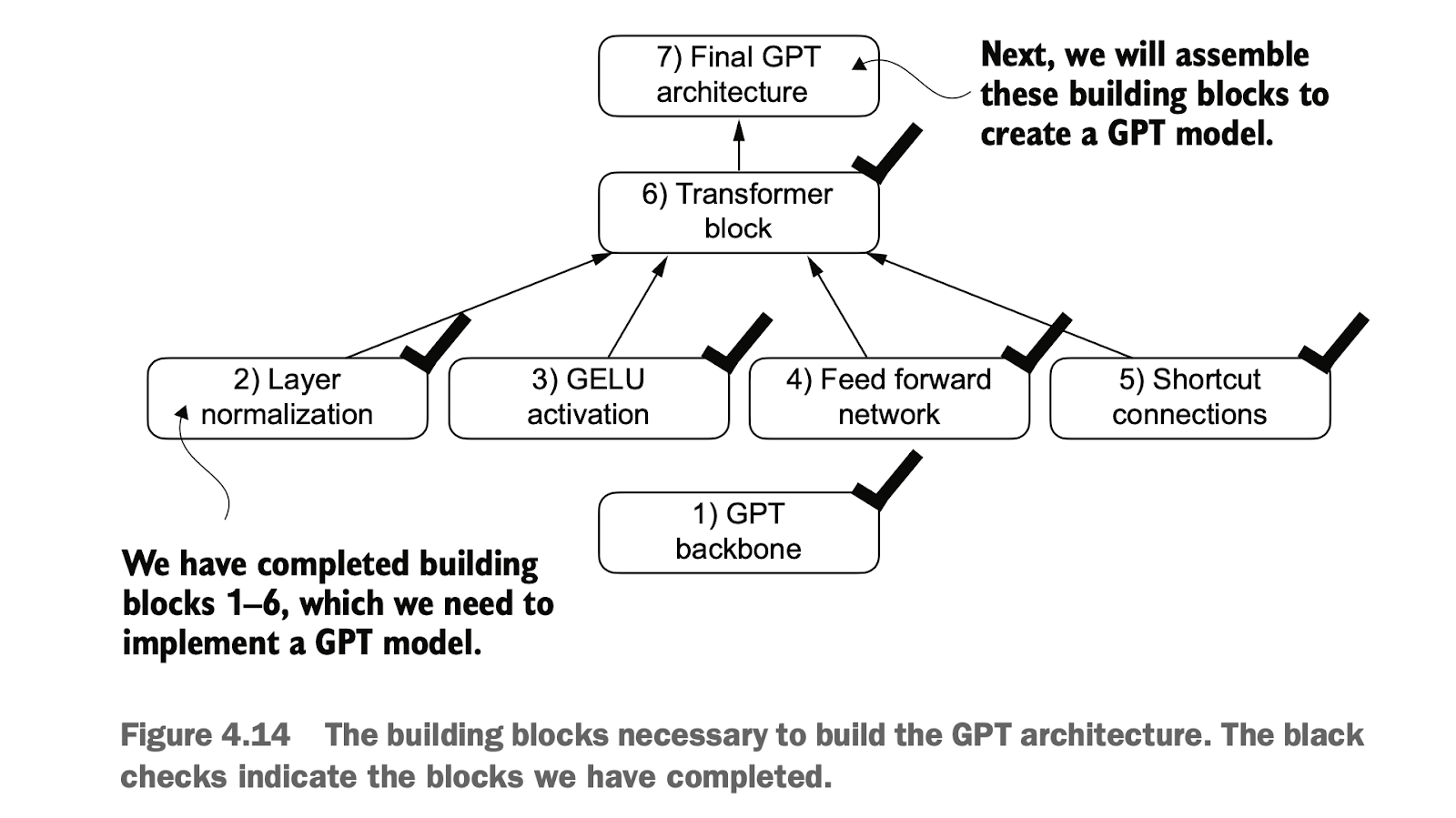
现在我们完成了构建 GPT 架构所需的所有组成部分。如图 ,Transformer 块结合了层归一化(Layer Normalization)、前馈网络(Feed Forward Network)、GELU 激活函数以及残差连接(Shortcut Connections)。
Now we have completed all the components required to build the GPT architecture. As shown, the Transformer block integrates layer normalization, feedforward networks, the GELU activation function, and shortcut connections.
4.6 完成GPT骨架编码 Completing the GPT Skeleton Encoding
完成了上面几个子模块的编码之后,我们接下来考虑将一开始骨架里的占位符替换成真正的模块
After completing the coding of the above submodules, the next step is to replace the placeholders in the initial skeleton with the actual modules.
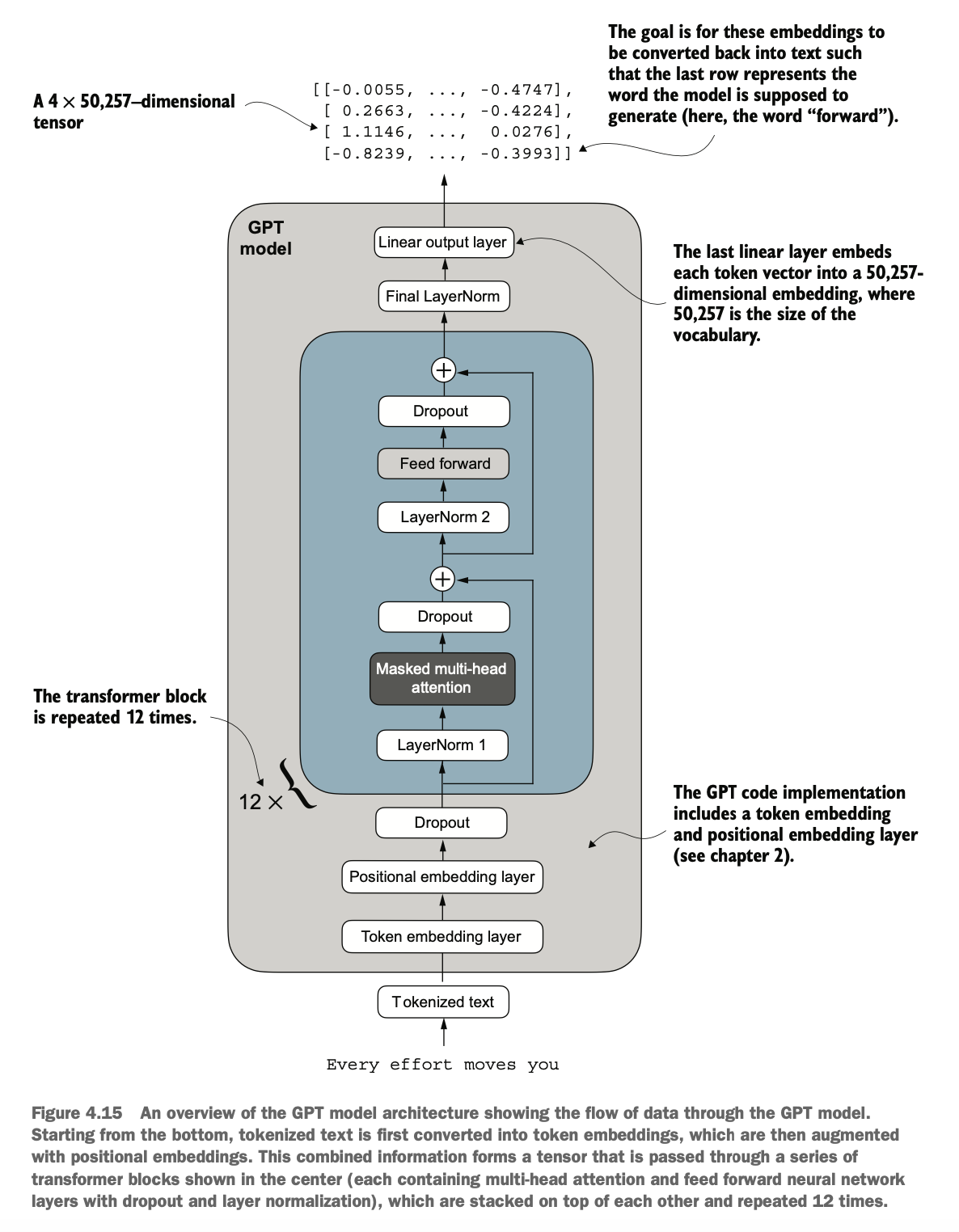
如图所示为一个GPT2模型简单架构
数据首先token化,然后使用位置向量增强和dropout
之后数据在transformer块重复处理了很多次(小GPT2重复了12次,大GPT2模型重复了48次)
最后token输出会映射到高纬度向量(如768维),之后再映射到词典的单词(如50257个单词),输出长度和输入长度一样,但表示往后偏移一位的预测,所以最后一个token是整个输入的输出预测token
As shown, the architecture of a simple GPT-2 model works as follows:
The input data is first tokenized and then enhanced using positional embeddings and dropout.
Next, the data is processed repeatedly through the Transformer blocks (12 times for small GPT-2, 48 times for large GPT-2).
Finally, the token outputs are mapped to high-dimensional vectors (e.g., 768 dimensions), which are then mapped to the vocabulary words (e.g., 50,257 words). The output length matches the input length but represents a prediction shifted one position forward. Therefore, the last token is the output prediction for the entire input sequence.
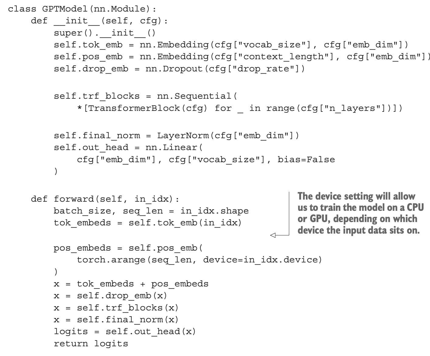
代码实现如下,
__init__ 方法:负责构建模型结构
初始化模型的核心模块:
创建 标记嵌入层(将输入标记索引转换为密集向量)。
创建 位置嵌入层(为输入序列添加位置信息)。
构建指定数量的 TransformerBlock 模块的堆叠。
添加 LayerNorm 层,用于标准化 Transformer 块的输出。
定义 线性输出头,将 Transformer 的输出映射到词汇表空间以生成 logits。
forward 方法:负责执行从输入到输出 logits 的前向计算过程
定义模型的前向传播逻辑:
接收输入标记索引并计算其 嵌入表示。
将位置嵌入添加到嵌入向量中。
将序列通过堆叠的 TransformerBlock 进行逐步处理。
对最终输出进行 归一化(LayerNorm)。
计算 logits,表示下一个标记的未归一化概率分布。
The implementation is as follows:
The __init__ method is responsible for constructing the model structure:
Initialize the core modules of the model:
Create a token embedding layer (to map input token indices to dense vectors).
Create a positional embedding layer (to add positional information to the input sequence).
Stack the specified number of TransformerBlock modules.
Add a LayerNorm to normalize the outputs of the Transformer blocks.
Define a linear output head to map the Transformer's output to the vocabulary space, generating logits.
The forward method is responsible for executing the forward computation process from input to output logits:
Define the forward propagation logic:
Receive input token indices and compute their embedded representations.
Add positional embeddings to the embedding vectors.
Process the sequence step by step through the stacked TransformerBlock.
Normalize the final output using LayerNorm.
Compute logits, representing the unnormalized probability distribution for the next token.
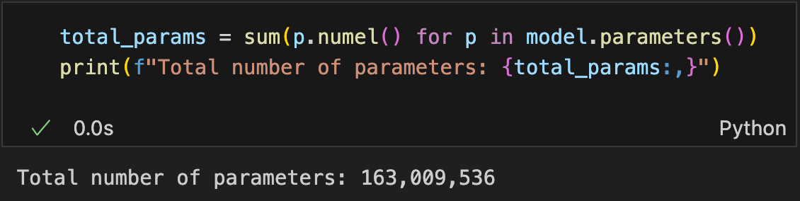
我们可以使用numel()方法打印参数个数,我们可以打印整个GPT模型的参数个数
We can use the numel() method to print the number of parameters in the model. This allows us to print the total number of parameters in the entire GPT model
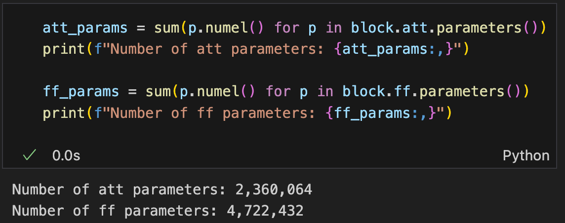
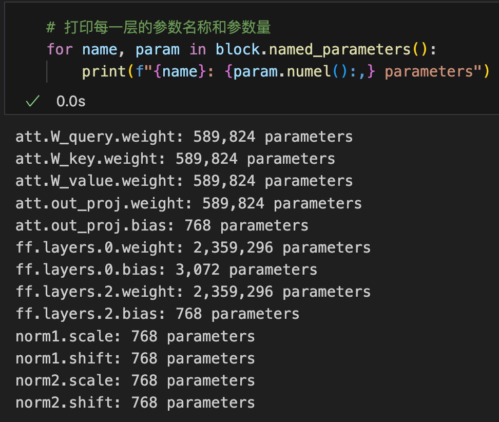
也可以查看transformer块里面的参数总个数和每个子模块的参数个数
as well as the total number of parameters within the Transformer blocks and each submodule.
注意,GPT2使用了权重共享(Weight Tying),即在模型中,标记嵌入层的权重(用于将输入标记映射为嵌入向量)和输出线性层的权重(用于将模型最终的高维向量映射回词汇表)是相同且共享的,即权重矩阵大小均为 [词汇表大小, 嵌入维度](如 [50257, 768])
Note that GPT-2 employs weight tying, meaning that the weights of the token embedding layer (used to map input tokens to embedding vectors) and the weights of the output linear layer (used to map the final high-dimensional vectors back to the vocabulary) are identical and shared. The size of the weight matrix is therefore [vocabulary size, embedding dimension] (e.g., [50257, 768]).
通过共享权重,可以显著减少模型的参数量,从而降低存储和计算成本,但实际上,如果使用分开不同的权重也可能会让模型表现更好(当然计算量也增加了)
By sharing weights, the total number of model parameters is significantly reduced, lowering storage and computational costs. However, using separate weights for these layers could potentially improve model performance, albeit with an increase in computational overhead.
根据算出来的模型参数个数,我们可以通过修改GPT模型参数配置以及使用一个float32作为一个参数的大小,预估GPT2对应的小、中、大尺寸模型(不使用权重共享情况下)大概要吃多少内存
小GPT2(768词维度,12层,12多头):163,009,536个参数,需要621.83 MB内存
中GPT2(1024词维度,24层,16多头):406,212,608个参数,需要1549.58 MB内存
大GPT2(1280词维度,36层,20多头):838,220,800个参数,需要3197.56 MB内存
加大GPT2(1600词维度,48层,25多头):1,637,792,000个参数,需要6247.68 MB内存
Based on the computed number of model parameters, we can estimate the memory consumption of GPT-2 models of various sizes (without weight sharing) by modifying the GPT model's parameter configuration and using 4 bytes (float32) per parameter:
Small GPT-2 (768 embedding dimension, 12 layers, 12 attention heads):
163,009,536 parameters, requiring 621.83 MB of memory.Medium GPT-2 (1024 embedding dimension, 24 layers, 16 attention heads):
406,212,608 parameters, requiring 1549.58 MB of memory.Large GPT-2 (1280 embedding dimension, 36 layers, 20 attention heads):
838,220,800 parameters, requiring 3197.56 MB of memory.Extra-Large GPT-2 (1600 embedding dimension, 48 layers, 25 attention heads):
1,637,792,000 parameters, requiring 6247.68 MB of memory.
4.7 使用GPT生成文本 Using GPT to Generate Text
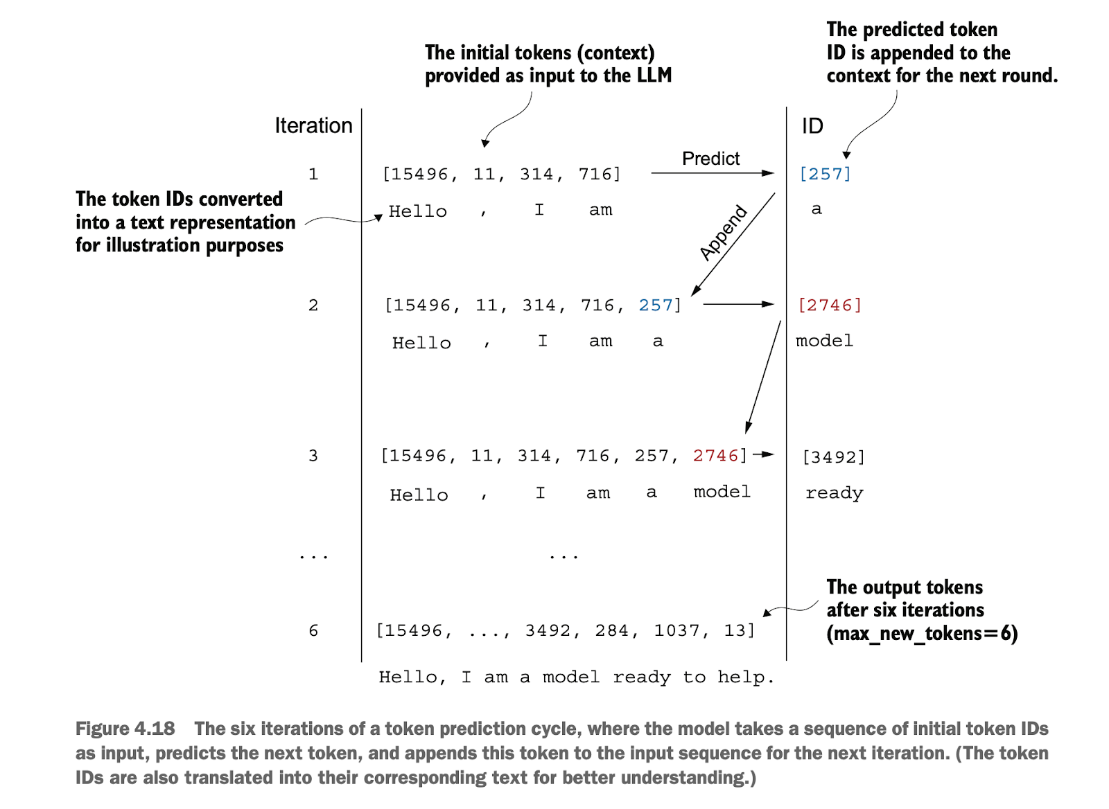
生成文本的原理很简单,通过一个一个单词的预测输出,最终弄成完整的一句话
The principle of text generation is straightforward: by predicting one word at a time, a complete sentence is eventually formed.
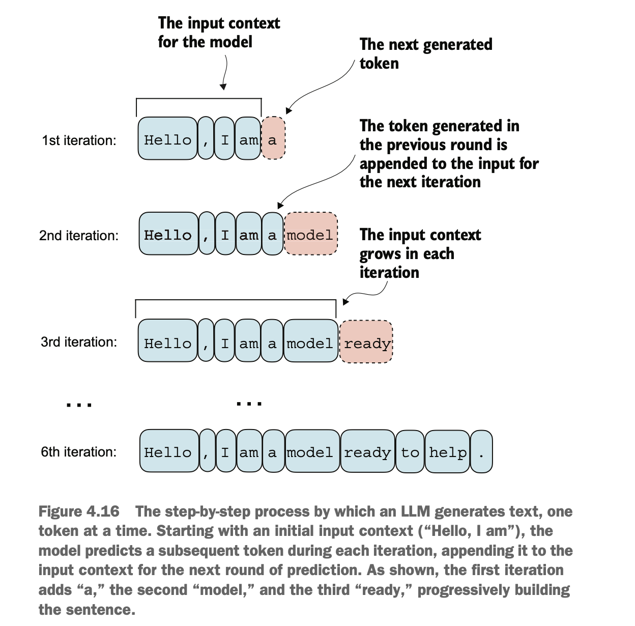
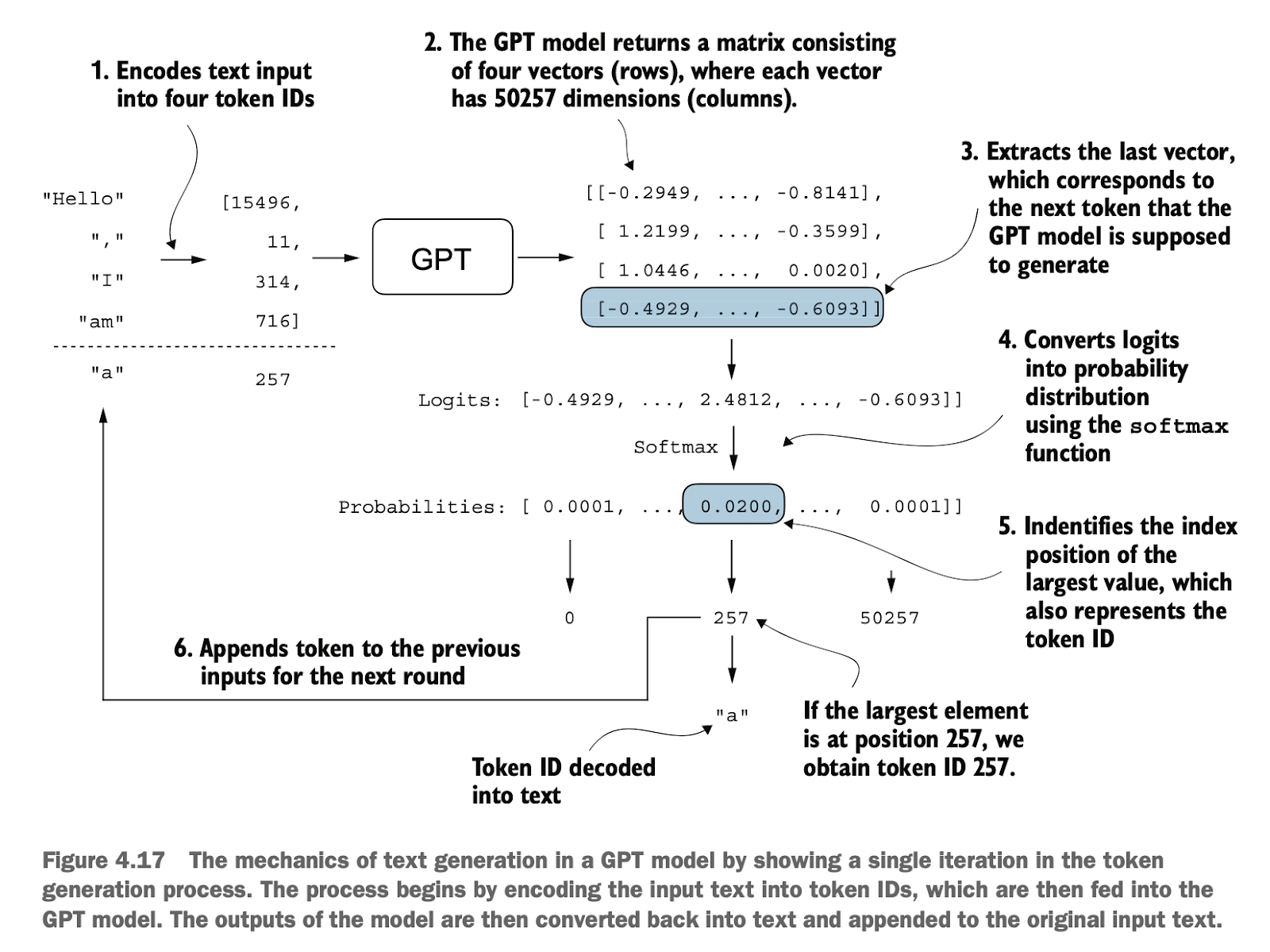
接下来,我们要将输出的[batch_size, num_token, vocab_size]数据转成人可读的文本,具体步骤如下:
编码输入:将输入文本转为对应的 token ID 列表(如 "Hello, I am" → [15496, 11, 314, 716])。
输入模型:把这些 token ID 输入到 GPT 模型中,模型输出一个矩阵(每行对应一个 token 的预测分布)。
取最后一行:选取最后一个 token 的输出 logits。
计算概率:使用 softmax 将 logits 转为概率分布。
确定下一个词:找到概率最大的那个索引,对应下一个 token ID(如 257)。
解码为文本:将 token ID 转为对应的文字(如 257 → "a")。
更新输入:将生成的词追加到输入序列中,作为下一轮的输入。
重复以上步骤:直到生成指定数量的词或达到结束条件。
Next, we need to convert the model's output data with the shape [batch_size, num_token, vocab_size] into human-readable text. The specific steps are as follows:
Encode the input: Convert the input text into a corresponding list of token IDs (e.g., "Hello, I am" → [15496, 11, 314, 716]).
Feed into the model: Input these token IDs into the GPT model, which outputs a matrix (each row corresponds to the predicted distribution for a token).
Take the last row: Select the output logits of the last token.
Compute probabilities: Use softmax to convert logits into a probability distribution.
Determine the next word: Find the index with the highest probability, which corresponds to the next token ID (e.g., 257).
Decode into text: Convert the token ID into its corresponding text (e.g., 257 → "a").
Update input: Append the generated word to the input sequence to be used as input for the next iteration.
Repeat the above steps: Continue until the specified number of words is generated or a stopping condition is met.
注意,这里因为softmax是单调函数,所以其实和不用softmax而是直接从logits中选最大的那个是一样的,但是我们后续可能会用其它的额外采样方式,并不一定选出概率最高的token,因为这样有利于变化性以及创造性
Note that because softmax is a monotonic function, it is essentially equivalent to directly selecting the largest value from the logits without applying softmax. However, in subsequent steps, we might use other sampling methods instead of always selecting the token with the highest probability, as this can improve variability and creativity in the generated text.
总结 Summary
层归一化通过确保每一层的输出具有一致的均值和方差来稳定训练过程。
快捷连接是跨过一层或多层的连接,通过将某一层的输出直接传递到更深层,从而缓解深度神经网络(如LLMs)训练中的梯度消失问题。
Transformer块是GPT模型的核心结构组件,它结合了带掩码的多头注意力模块和使用GELU激活函数的全连接前馈网络。
GPT模型是具有大量重复Transformer块的LLMs,其参数规模从数百万到数十亿不等。
GPT模型有多种规模,例如124、345、762和1,542百万参数,这些模型可以通过同一个GPTModel Python类来实现。
GPT类LLM的文本生成能力通过逐步预测一个个token(标记),将输出张量解码成可读文本,并基于给定的输入上下文进行。
如果没有经过训练,GPT模型会生成不连贯的文本,这突出了模型训练对于生成连贯文本的重要性。
Layer normalization stabilizes the training process by ensuring that each layer's output has consistent mean and variance.
Shortcut connections skip over one or more layers, directly passing a layer's output to deeper layers. This alleviates the vanishing gradient problem during the training of deep neural networks (e.g., LLMs).
Transformer blocks are the core structural components of GPT models, combining masked multi-head attention modules with fully connected feedforward networks using the GELU activation function.
GPT models are LLMs with a large number of repeated Transformer blocks, with parameter scales ranging from millions to billions.
GPT models come in various sizes, such as 124M, 345M, 762M, and 1,542M parameters, all of which can be implemented using the same GPTModel Python class.
The text generation capability of GPT-like LLMs relies on token-by-token predictions, decoding the output tensor into readable text based on the given input context.
Without proper training, GPT models generate incoherent text, highlighting the importance of training for producing coherent and meaningful outputs.