降维算法原理 Dimensionality Reduction Algorithm Principles

背景 Background 

如果拿到的数据特征过于庞大，一方面会使得计算任务变得繁重;另一方面，如果数据特征还有问 题，可能会对结果造成不利的影响。降维是机器学习领域中经常使用的数据处理方法，一般通过某种映 射方法，将原始高维空间中的数据点映射到低维度的空间中，本章将从原理和实践的角度介绍两种经典 的降维算法——LDA线性判别分析和PCA主成分分析。

If the features of the obtained data are too large, on one hand, it will make the computational tasks more burdensome; on the other hand, if there are issues with the data features, it may negatively affect the results. Dimensionality reduction is a commonly used data processing method in the field of machine learning. Typically, through some form of mapping, data points in the original high-dimensional space are mapped to a lower-dimensional space. This chapter will introduce two classic dimensionality reduction algorithms—Linear Discriminant Analysis (LDA) and Principal Component Analysis (PCA)—from both theoretical and practical perspectives.

15.1 线性判别分析LDA.pdf

15.2 主成分分析PCA.pdf

线性判别式分析(Linear Discriminant Analysis,LDA) 

原理 Principle

假设有两类数据点，如图15-2所示。由于数据点都是二维特征， 需要将其降到一维，也就是需要找到一个最合适的投影方向把这些数据点全部映射过去。图(a)、 (b)分别是选择两个投影方向后的结果，那么，究竟哪一个更好呢?

Assume there are two classes of data points, as shown in Figure 15-2. Since the data points have two-dimensional features, we need to reduce them to one dimension. In other words, we need to find the most suitable projection direction to map all of these data points. Figure (a) and Figure (b) show the results of selecting two different projection directions. So, which one is better?

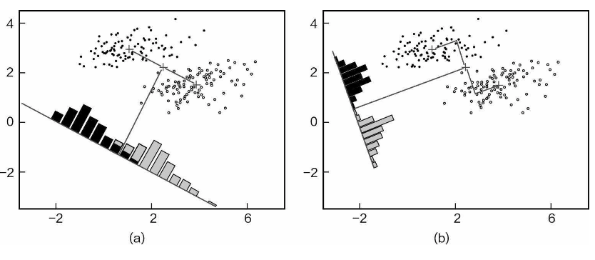
从投影结果上观察，图(a)中的数据点经过投影后依旧有一部分混在一起，区别效果有待提 高。图(b)中的数据点经过投影后，没有混合，区别效果比图(a)更好一些。因此，我们当然 会选择图(b)所示的降维方法，由此可见，降维不仅要压缩数据的特征，还需要寻找最合适的方 向，使得压缩后的数据更有利用价值。

From the projection results, in Figure (a), some data points are still mixed together after projection, and the distinction between the two classes could be improved. In contrast, in Figure (b), the data points are not mixed after projection, and the distinction is clearer compared to Figure (a). Therefore, we would naturally choose the dimensionality reduction method shown in Figure (b). This demonstrates that dimensionality reduction not only needs to compress the data's features, but also needs to find the most suitable direction, so that the compressed data is more useful.

为了把降维任务做得更圆满，实现“尽可能使两类数据点区别得越明显越好，不要混在一起”的目的，提出了两个目标：

To perform dimensionality reduction more effectively and achieve the goal of “making the two classes of data points as distinguishable as possible without mixing together,” two objectives are proposed:

目标1. 对于不同类别的数据点，希望其经过投影后能离得越远越好。（不同类分散）

目标2. 对于同类别的数据点，希望它们能更集中，离组织的中心越近越好。（同类集中）

Objective 1: For data points of different classes, we hope that after projection, they are as far apart as possible. (Inter-class dispersion)

Objective 2: For data points of the same class, we want them to be more concentrated and as close to the center of their cluster as possible. (Intra-class compactness)

接下来的任务就是完成这两个目标，这也是线性判别分析的核心优化目标，降维任务就是找到能同 时满足这两个目标的投影方向。

The next task is to achieve these two objectives, which is the core optimization goal of Linear Discriminant Analysis (LDA). The dimensionality reduction task is to find a projection direction that satisfies both objectives simultaneously.

求解和计算 Solving and Calculation

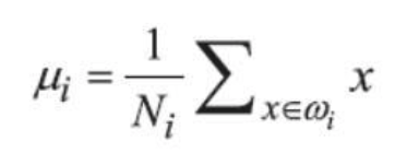
要定义一下距离这个 概念，例如“扎堆”该怎么体现呢?这里用数据点的均值来表示其中心位置，如果每一个数据点都离中心 很近，它们就“扎堆”在一起了。中心点位置计算方法如下:

First, we need to define the concept of "distance." For instance, how do we quantify "clustering" or "gathering"? Here, the mean of the data points is used to represent the central position. If each data point is very close to the center, they are "clustered" together. The method for calculating the center point is as follows:

在降维算法中，其实我们更关心的并不是原始数据集中数据点的扎堆情况，而是降维后的结果，因此，可知投影后中心点位置为:

In dimensionality reduction algorithms, we are not as concerned with the clustering of data points in the original dataset, but rather with the result after dimensionality reduction. Therefore, the center point after projection can be determined as:

我们还可以使用另一个度量指标——散列值(scatter)，表示同类数据样本点的离散程度，定义如下:

We can also use another metric called the scatter value, which represents the degree of dispersion of data points from the same class. The scatter is defined as follows:

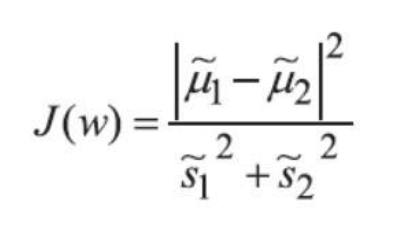
优化的目标有两个，那么如何才能整合它们呢?既然要最大化不同类别之间的距离，那就把它当作分子;最小化同类样本之间的离散程度，那就把 它当作分母，最终整体的J(W)依旧求其极大值即可。

Since there are two optimization objectives, how can we integrate them? Given that we want to maximize the distance between different classes, we can treat that as the numerator. On the other hand, we want to minimize the dispersion among samples of the same class, so we can treat that as the denominator. Ultimately, the overall objective function J(W) will seek to maximize this ratio.

这里需要先求出类内散布矩阵和类间散布矩阵

Here, we first need to calculate the within-class scatter matrix and the between-class scatter matrix.

然后使用拉格朗日乘子法推导，得到

Then, using the Lagrange multiplier method for derivation, we obtain:

观察一下式，它与线性代数中的特征向量有点像，如果把当作一个整体，那么w就是其特征向量，问题到此迎刃而解。在线性判别分析中，其实只需要得到类内和类间散布矩阵，然后求其特征向量，就可以得到投影方向，然后，只需要对数据执行相应的矩阵变换，就完成全部降维操作。

If we observe this equation, it looks somewhat similar to the eigenvector formulation in linear algebra. If we treat  as a whole, then w is its eigenvector. At this point, the problem is essentially solved. In Linear Discriminant Analysis (LDA), all we need to do is obtain the within-class and between-class scatter matrices, then compute their eigenvectors to find the projection directions. Afterward, by performing the corresponding matrix transformation on the data, the entire dimensionality reduction process is completed. 

注意，根据线性判别分析（LDA）的原理，投影的维度数 n_components 不能超过 min(n_features, n_classes - 1)

An important note: according to the principles of LDA, the number of projection dimensions n_components cannot exceed min(n_features, n_classes - 1)

代码 Code

下面要在非常经典的“鸢尾花”数据集上使用线性判别分析完成降维任务。数据集中含有3 类、共150条鸢尾花基本数据，其中山鸢尾、变色鸢尾、维吉尼亚鸢尾各有50条数据，每条数据包括萼片 长度(单位:厘米)、萼片宽度、花瓣长度、花瓣宽度4种特征。数据集共有150条数据，每条数据有4个特征，现在需要将四维特征降成二维。

Next, we will use Linear Discriminant Analysis (LDA) to perform dimensionality reduction on the very classic "Iris" dataset. The dataset contains 3 classes with a total of 150 Iris flower data points: 50 each for Setosa, Versicolor, and Virginica. Each data point includes 4 features: sepal length (in cm), sepal width, petal length, and petal width. The dataset has 150 data points, each with 4 features, and we need to reduce these four-dimensional features to two dimensions.

from sklearn.preprocessing import LabelEncoder

feature_dict = {i:label for i,label in zip(
                range(4),
                  ('sepal length in cm',
                  'sepal width in cm',
                  'petal length in cm',
                  'petal width in cm', ))}
label_dict = {i:label for i,label in zip(
                range(1,4),
                  ('Setosa',
                  'Versicolor',
                  'Virginica'
                 ))}
df = pd.io.parsers.read_csv(
    filepath_or_buffer='https://archive.ics.uci.edu/ml/machine-learning-databases/iris/iris.data',
    header=None,
    sep=',',
    )

X = df[['sepal length in cm','sepal width in cm','petal length in cm','petal width in cm']].values
y = df['class label'].values

from sklearn.discriminant_analysis import LinearDiscriminantAnalysis as LDA

# 调用包实现LDA
sklearn_lda = LDA(n_components=2)
X_lda_sklearn = sklearn_lda.fit_transform(X, y)

# 查看结果 check result
print(X_lda_sklearn.shape)
print("特征值（explained_variance_ratio_）: ", sklearn_lda.explained_variance_ratio_)
print("特征向量（scalings_）: ", sklearn_lda.scalings_)

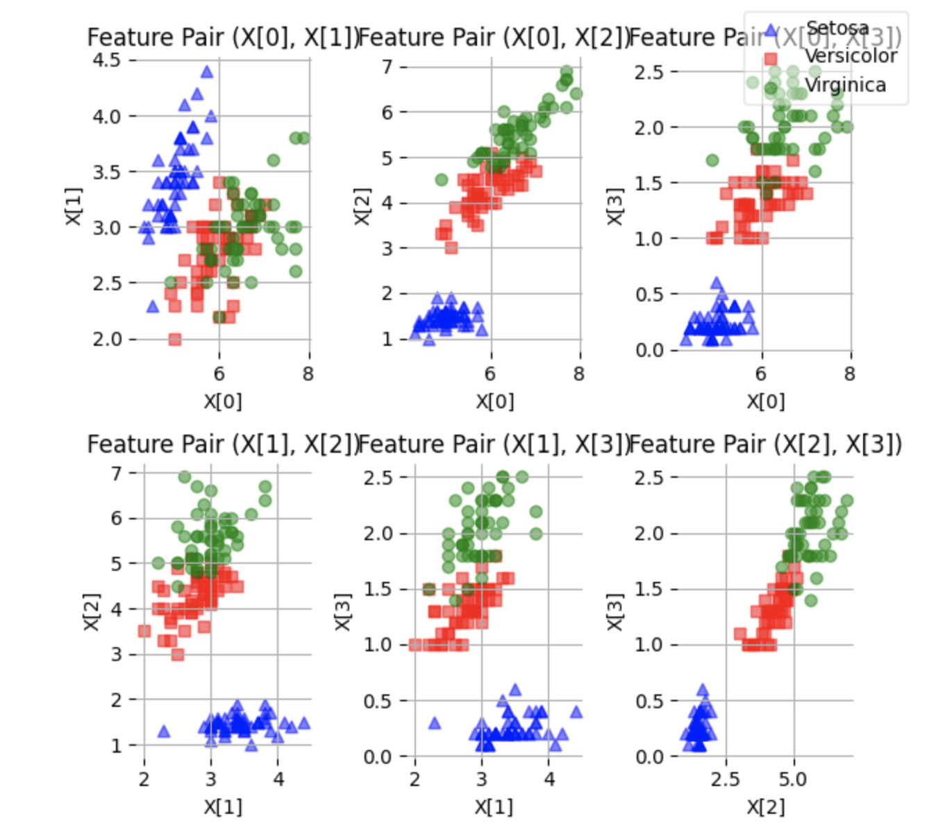
现在可以看到数据维度从原始的(150,4)降到(150,2)，到此就完成全部的降维工作。接下来对比 分析一下降维后结果，为了方便可视化展示，在原始四维数据集中随机选择两维进行绘图展示:

Now, we can see that the data dimensions have been reduced from the original (150, 4) to (150, 2), thus completing the dimensionality reduction process. Next, let's compare and analyze the results after dimensionality reduction. For easier visualization, we will randomly select two dimensions from the original four-dimensional data for plotting:

选取降到2维后的数据进行可视化：

Visualizing the reduced 2D data:

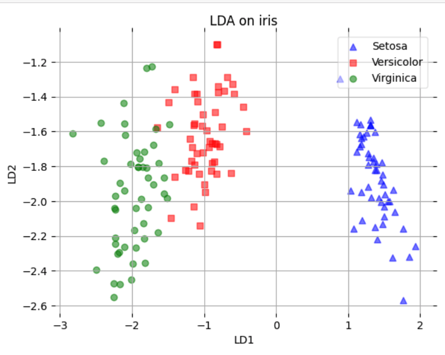
可以明显看到，坐标轴变成LD1与LD2，这就是降维后的结果，从数据点的分布来看，混杂在一起的数据不多，划分起来就更容易。这就是经过一步步计算得到的最终降维结果。

You can clearly see that the axes have become LD1 and LD2, which represent the reduced dimensions. From the distribution of the data points, we can observe that there is little overlap among the classes, making it easier to separate them. This is the final result of the dimensionality reduction obtained through step-by-step calculations.

主成分分析(Principal Component Analysis，PCA)

原理 Principle

主成分分析(Principal Component Analysis，PCA)是在降维中使用特别广泛的算法。在使用主成分分析降维的时候没有束缚，不像线性判别分析，必须要有数据标签，只要拿到数据，没有标签也可以用 主成分分析进行降维。所以应该先有一个直观的认识，主成分分析本质上属于无监督算法，这也是它流行的主要原因。

Principal Component Analysis (PCA) is a widely used algorithm for dimensionality reduction. Unlike Linear Discriminant Analysis (LDA), PCA does not require labeled data, making it more flexible for unsupervised learning tasks. You can apply PCA to a dataset even if it lacks labels, which is one of the reasons for its popularity.

考虑将一组二维数据进行降维，如何选取这个一维坐标系使得能保留的信息最多呢？如果降维后都到同一个点，那就没有保留任何信息，而要保留更多的信息，就得尽可能有区分度（方差尽可能大）。

PCA aims to reduce the dimensionality of the data while preserving as much variance (information) as possible. For example, when reducing a set of two-dimensional data to one dimension, the goal is to select a projection that retains the maximum variance. If all data points are projected onto the same point, no information is preserved. Therefore, in PCA, the projection should maximize the variance to ensure that the most distinguishing information is retained.

推荐一个B站视频：https://www.bilibili.com/video/BV1E5411E71z

I recommend watching this Bilibili video: https://www.bilibili.com/video/BV1E5411E71z

求解和计算 Solving and Calculation

推导前需要补充下方差和协方差的概念。方差(variance)相当于特征辨识度，其值越大越好。协方差(covariance)就 是不同特征之间的相关程度，协方差的计算式为:

Before proceeding with the derivation, it's important to introduce the concepts of variance and covariance. Variance represents the distinguishability of a feature; the larger its value, the better. Covariance describes the degree of correlation between different features, and its formula is:

如果两个变量的变化趋势相同，例如随着身高的增长，体重也增长，此时它们的协方差值就会比较 大，表示正相关。而方差又描述了各自的辨识能力。

If two variables have similar trends, for example, as height increases, weight increases as well, their covariance will be large, indicating a positive correlation. Variance, on the other hand, describes the distinguishability of each feature individually.

要推导出这个降维的新坐标，首先要去中心化（把坐标原点放在数据的中心）即将每个特征的均值变为0，得到中心化后的数据矩阵X~。

To derive this new coordinate system for dimensionality reduction, the first step is centering the data (i.e., placing the origin of the coordinate system at the center of the data). This is done by subtracting the mean from each feature, so that the mean of each feature becomes 0. The result is the centered data matrix X~ .

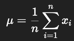
然后需要计算协方差矩阵，计算出特征向量（新坐标的坐标轴方向）和特征值（新坐标轴方向的方差）

Next, the covariance matrix needs to be computed, which is then used to calculate eigenvectors (the directions of the new coordinate axes) and eigenvalues (the variance along these new axes).

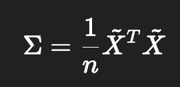
接下来要找到数据集的主成分，即数据在某些方向上的方差最大。主成分对应协方差矩阵 Σ Σ 的特征向量。具体地，PCA通过对协方差矩阵 ΣΣ 进行特征值分解来完成：

The goal is to find the principal components of the dataset, i.e., the directions in which the variance of the data is maximized. The principal components correspond to the eigenvectors of the covariance matrix ΣΣ. Specifically, PCA is accomplished by performing eigenvalue decomposition on the covariance matrix ΣΣ:

其中U是是协方差矩阵的特征向量矩阵，每一列是一个特征向量（表示方差最大下新坐标系的坐标轴），中间是是对角矩阵，对角线上元素是对应的特征值，表示数据沿着相应特征向量方向的方差大小（该新坐标轴方向的方差）

where U is the eigenvector matrix of the covariance matrix, with each column representing an eigenvector (indicating the direction of the axes in the new coordinate system where variance is maximized), and Λ is a diagonal matrix whose diagonal elements are the eigenvalues, representing the variance along the corresponding eigenvector direction (i.e., the variance along that new coordinate axis).

之后，我们可将特征值按照从大到小的顺序排列，选择其中较大的K个主成分，然后将其对应的K个特征向量组成投影矩阵

Next, we arrange the eigenvalues in descending order and select the top K principal components. We then form a projection matrix from the corresponding K eigenvectors

如此一来，通过PCA，我们可以从高维数据中提取出方差最大的方向，保留数据的主要信息，同时减少维度

Thus, through PCA, we can extract the directions of maximum variance from high-dimensional data, preserving the most important information while reducing the dimensionality.

代码 Code

接下来通过一个实例介绍如何使用PCA处理实际问题，同样使用鸢尾花数据集，目的依旧是完成降维任务

Next, let's introduce how to use PCA to solve a real-world problem, using the Iris dataset once again. The goal remains the same: to complete the task of dimensionality reduction

import numpy as np
import pandas as pd

df = pd.read_csv('iris.data')
df.columns=['sepal_len', 'sepal_wid', 'petal_len', 'petal_wid', 'class']
df.head()

完成数据的标准化

Standardizing the Data

X = df.iloc[:,0:4].values
y = df.iloc[:,4].values

from sklearn.preprocessing import StandardScaler
X_std = StandardScaler().fit_transform(X)

展示数据特征

Displaying Data Features

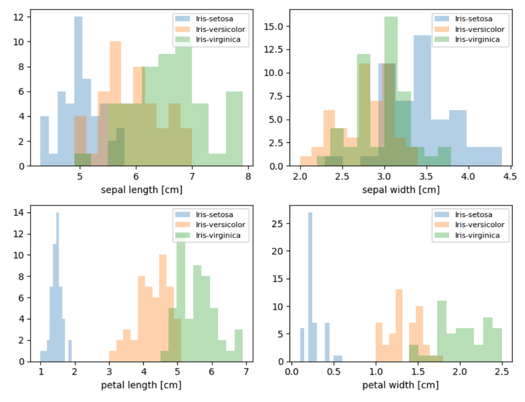
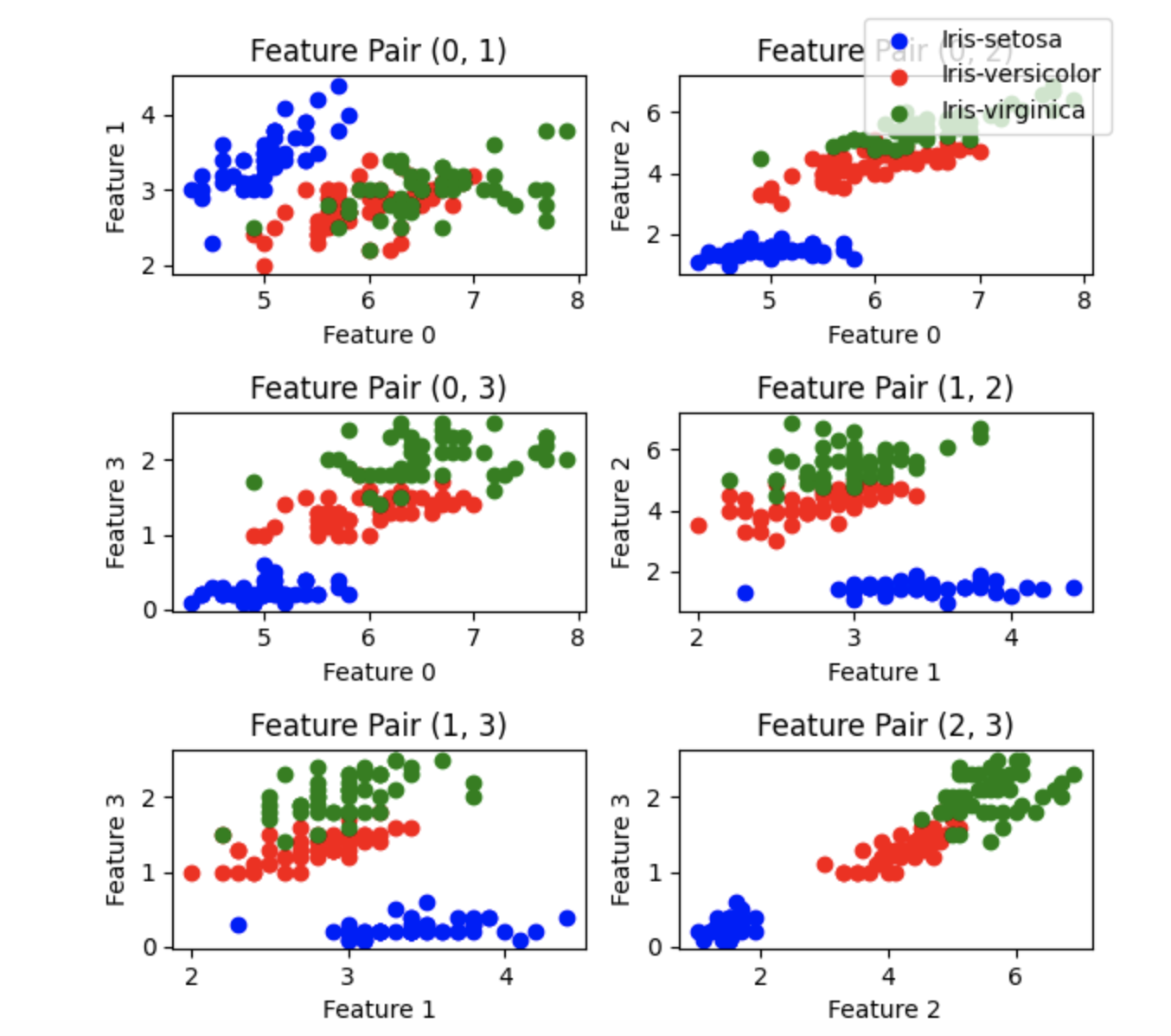
可以看出，有些特征区别能力较强，能把3种花各自呈现出来;有 些特征区别能力较弱，部分特征数据样本混杂在一起。

You can see that some features have strong distinguishing ability, clearly separating the three different types of flowers; however, some features are less effective at distinguishing the flowers, as certain samples are mixed together.

直接使用Numpy工具包来计算协方差

We now calculate the covariance matrix using the Numpy library.

np.cov(X_std.T)

求特征值与特征向量

Calculating Eigenvalues and Eigenvectors

cov_mat = np.cov(X_std.T)
eig_vals, eig_vecs = np.linalg.eig(cov_mat)
print('特征向量 \n%s' %eig_vecs)
print('\n特征值 \n%s' %eig_vals)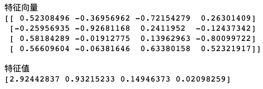

可以发现，使用前两个特征值时，其对应的累计贡献率已经超过95%，所以选择降到二维。接下来把特征向量组合起来完成降维工作:

Upon calculation, we find that by using the first two eigenvalues, the cumulative explained variance exceeds 95%. Therefore, we choose to reduce the data to two dimensions. Next, we combine the eigenvectors to complete the dimensionality reduction:

matrix_w = np.hstack((eig_pairs[0][1].reshape(4,1),
                      eig_pairs[1][1].reshape(4,1)))
print('Matrix W:\n', matrix_w)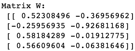

Y = X_std.dot(matrix_w)

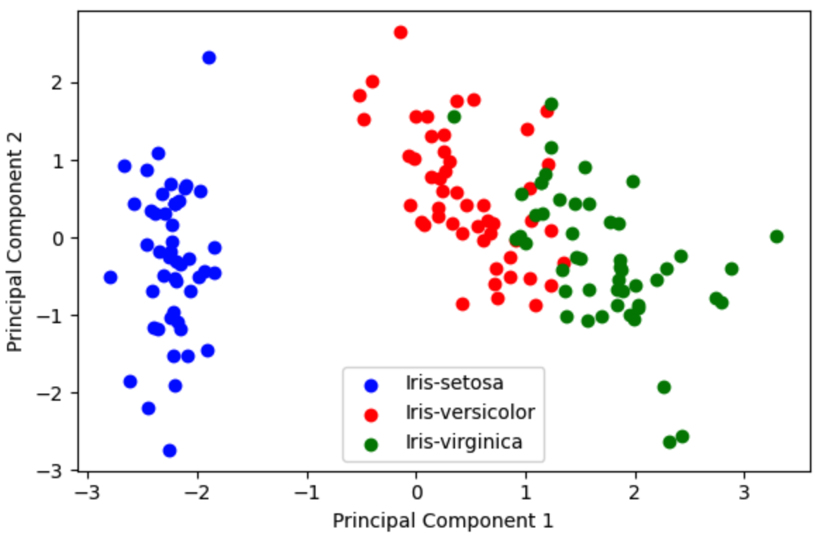
这样，我们就使用了PCA降维算法把原数据矩阵从150×4降到150×2

In this way, we have used the PCA dimensionality reduction algorithm to reduce the original data matrix from 150×4 to 150×2

这时我们可以进行可视化对比降维前后数据的分布。由于数据具有4个特征，无法在平面图中显示，因此只使用两维特征显示数据

At this point, we can visualize and compare the data distribution before and after dimensionality reduction. Since the data has four features, it cannot be fully displayed in a 2D plot. Therefore, we will only display two of the features.

只使用前两个特征显示3类数据，如图15-11所示，看起来3类鸢尾花相互交叠在一起，不容易区分开，下面看看使用PCA降维后的情况：

By showing only the first two features, the three types of flowers (Iris) appear to overlap, making it difficult to distinguish them, as shown in Figure 15-11. Now, let's see what happens after applying PCA for dimensionality reduction:

对比和总结 Comparison and Conclusion

本章介绍了两种非常实用的降维方法:线性判别分析和主成分分析。其中线性判别分析是有监督算 法，需要有标签才能计算;而主成分析是无监督算法，无须标签，直接就可以对数据进行分析。那么， 在实际建模任务中，到底用哪种降维方法呢?没有固定的模式，需要大家通过实验对比确定，例如，取 得一份数据后可以分多步走，以对比不同策略的结果。

This chapter introduced two very practical dimensionality reduction methods: Linear Discriminant Analysis (LDA) and Principal Component Analysis (PCA). LDA is a supervised algorithm, requiring labels to compute, while PCA is an unsupervised algorithm, which can analyze data directly without needing labels. So, which dimensionality reduction method should be used in real modeling tasks? There is no fixed rule. It depends on experimentation and comparison to determine the best approach. For example, after obtaining a dataset, you can proceed step by step to compare the results of different strategies.

PCA（主成分分析）的目标是最大化总方差。它寻找数据中方差最大的方向，而忽略类别信息。换句话说，PCA 的目的是找到那些在所有样本中变化最多的方向，而不关心不同类别之间的区分。所以，PCA降维后，可能无法很好地区分类别。

LDA（线性判别分析）的目标是最大化类间方差与类内方差的比率，即它试图找到一个投影方向，使得不同类别之间的分离最大化。因此，LDA 是专门为分类问题设计的降维方法，通常在分类任务中表现更好。

PCA (Principal Component Analysis) aims to maximize the total variance. It looks for the directions in the data with the largest variance, while ignoring class information. In other words, the purpose of PCA is to find the directions where the data varies the most across all samples, without considering the distinctions between different classes. Therefore, after dimensionality reduction with PCA, it may not effectively separate categories.

LDA (Linear Discriminant Analysis), on the other hand, aims to maximize the ratio of between-class variance to within-class variance. It seeks to find a projection direction that maximizes the separation between different categories. As a result, LDA is a dimensionality reduction method specifically designed for classification tasks and typically performs better in such tasks.

SVD分解和PCA主成分的关系 

Relationship between SVD decomposition and PCA principal components

这里可以补充一下，SVD分解和PCA主成分的关系：

• PCA 的主成分方向：可由 SVD的矩阵V的列向量（右奇异向量）给出。

• PCA 中的特征值：由 SVD 分解中的奇异值的平方给出。奇异值越大，表示数据在对应主成分方向上的方差越大。

• 降维：通过 SVD 得到的主成分，可以用于将原始数据投影到低维空间（即使用前  k 个主成分），这就是 PCA 中的降维过程。

• 好处：在利用SVD分解可以不用求协方差的情况下求出主成分V和奇异值

例如，在用户评分矩阵的 SVD 分解中，矩阵 Vt 可以理解为商品的隐含特征，而这些隐含特征在 PCA 的框架下确实可以看作是商品的 主成分

Here, we can supplement the relationship between SVD decomposition and PCA principal components:

• Principal component directions in PCA: These can be obtained from the column vectors of the matrix V (right singular vectors) in SVD decomposition.

• Eigenvalues in PCA: These are given by the squares of the singular values from SVD decomposition. The larger the singular value, the greater the variance of the data in the corresponding principal component direction.

• Dimensionality reduction: The principal components obtained from SVD can be used to project the original data into a lower-dimensional space (i.e., using the first k principal components). This is the dimensionality reduction process in PCA.

• Benefit: By using SVD decomposition, you can directly obtain the principal components V and singular values without needing to compute the covariance matrix.

For example, in the SVD decomposition of a user rating matrix, the matrix Vt can be understood as the implicit features of the items. These implicit features, within the framework of PCA, can indeed be considered as the principal components of the items.