聚类算法原理 Clustering Algorithms Principles

背景 Background 

分类和回归算法在推导过程中都需要数据标签，也就是有监督问题。那么，如果数据本身没有标 签，如何把它们按堆进行划分呢?这时候聚类算法就派上用场了

Classification and regression algorithms both require data labels during the derivation process, which makes them supervised learning problems. But what if the data itself doesn't have labels? How can we group the data into clusters? This is where clustering algorithms come into play.

K-means算法 K-means Clustering

K-means是聚类算法中最经典、最实用，也是最简单的代表，它的基本思想直截了当，效果也不错

K-means is the most classic, practical, and also the simplest representative of clustering algorithms. Its basic idea is straightforward, and the performance is quite good.

步骤 Steps

1. 选择 K 值：指定要生成的聚类的数量，即选择 K 个聚类的中心点（质心）。

2. 初始化质心：随机选择 K 个数据点作为初始质心。质心是聚类的中心，用来表示每个聚类的中心位置。

3. 分配数据点到最近的质心：

    对每个数据点，计算它到所有质心的距离（通常使用欧氏距离）。

    将每个数据点分配到距离最近的质心所对应的聚类中。

4. 更新质心：

    重新计算每个聚类的质心，质心是该聚类中所有数据点的平均值。

5. 重复步骤 3 和 4：

    重复分配数据点并更新质心的过程，直到质心不再变化（或变化非常小），或者达到指定的迭代次数。

6. 算法终止：当质心不再发生显著变化或达到最大迭代次数时，算法停止。

1. Choose the value of K: Specify the number of clusters to generate, that is, select K cluster centroids (centers).

2. Initialize centroids: Randomly select K data points as the initial centroids. A centroid is the center of a cluster and represents the central position of each cluster.

3. Assign data points to the nearest centroid:

    For each data point, calculate its distance to all centroids (usually using Euclidean distance).

    Assign each data point to the cluster corresponding to the closest centroid.

4. Update centroids:

    Recalculate the centroid of each cluster. The centroid is the average of all data points within that cluster.

5. Repeat steps 3 and 4:

    Repeat the process of assigning data points and updating centroids until the centroids no longer change (or change very little), or until the specified number of iterations is reached.

6. Algorithm termination: The algorithm stops when the centroids no longer change significantly or when the maximum number of iterations is reached.

相关参数 Relevant Parameters

(1) K值的确定。K值决定了待分析的数据会被划分成几个簇

(2) 质心的选择。选择适当的初始质心是K-means算法的关键步骤，通常都是随机给出，那么如果初始时选择的质心不同，或者说每一次执行K-means后的结果都相同吗?大部分情 况下得到的结果都是一致的，但不能保证每次聚类的结果都相同

(3) 距离的度量。常用的距离度量方法包括欧氏距离和余弦相似度等。距离的选择也可以当作是K- means的一种参数，不同度量方式会对结果产生不同的影响

(4) 评估方法。聚类算法由于本身的无监督性，没法用交叉验证来评估结果，只能大致观察结果的 分布情况。轮廓系数(Silhouette Coefficient)是聚类效果好坏的一种评价方式，也是最常用的评估方法

1. Determining the value of K: The value of K determines how many clusters the data will be divided into during the analysis.

2. Selection of centroids: Choosing appropriate initial centroids is a key step in the K-means algorithm. Typically, centroids are selected randomly. So, what happens if different centroids are chosen initially? Will the results be the same each time K-means is executed? In most cases, the results are consistent, but there is no guarantee that the clustering results will be the same every time.

3. Distance measurement: Common methods for measuring distance include Euclidean distance and cosine similarity. The choice of distance metric can be considered a parameter of K-means, as different metrics can affect the results in different ways.

4. Evaluation method: Due to the unsupervised nature of clustering algorithms, cross-validation cannot be used to evaluate the results. Instead, the distribution of the results can be roughly observed. The Silhouette Coefficient is one of the most commonly used methods to assess the quality of clustering, serving as a standard for evaluating clustering performance.

实际应用场景 Real-World Application Scenario

手头有一份国会投票的数据114_congress.csv，数据集中有100行，表示100名议员的投票。当前分析目标：因为民主党和共和党投票上有不同风格，根据他们的投票分2类验证是否如此，并找出投票异常的议员

We have a dataset titled 114_congress.csv, which contains voting data from Congress. The dataset consists of 100 rows, representing the votes of 100 legislators. The goal of the current analysis is to determine if there are distinct voting patterns between Democrats and Republicans by clustering their votes into 2 groups, thereby verifying this hypothesis. Additionally, we aim to identify any legislators with abnormal voting behavior.

数据集中有18列，分别是：

• name:议员的名字

• party:议员的党派（D代表民主党，R代表共和党，I表示无党派）

• state:议员所在的州

• 00001, 00004, 00005 等列是议员在不同议案（法案）上的投票结果，总共涉及 15 个议案

The dataset has 18 columns, which are as follows:

• name: The name of the legislator

• party: The party affiliation of the legislator (D for Democrat, R for Republican, and I for Independent)

• state: The state that the legislator represents

• Columns like 00001, 00004, 00005, etc., represent the voting results of the legislators on various bills, covering a total of 15 bills.

每个议员对多个法案的投票情况以 0、1 和 0.5 表示：

• 0 可能表示反对某个法案

• 1 可能表示支持某个法案

• 0.5 可能表示弃权或未投票

Each legislator's vote on multiple bills is represented by the values 0, 1, and 0.5:

• 0 likely represents opposition to a bill

• 1 likely represents support for a bill

• 0.5 likely represents abstention or absence from voting

votes = pd.read_csv("./114_congress.csv")
print(votes.shape)
votes

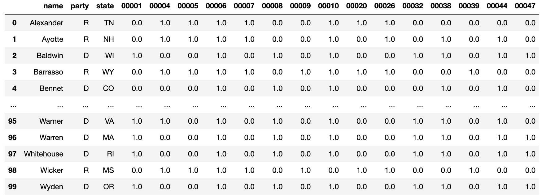
 使用K-means把数据分到2个类里，计算质心，把每个议员到两个质心的距离算出来，存到class2_x和class2_y中

Using K-means, we group the data into 2 clusters, compute the centroids, and calculate the distance of each legislator to the two centroids, storing these distances in class2_x and class2_y.

# use K-means to create 2 clusters
from sklearn.cluster import KMeans

numeric_votes = votes.drop(['name', 'party', 'state'], axis=1)
kmeans2 = KMeans(n_clusters=2, random_state=42)
votes['class2'] = kmeans2.fit_predict(numeric_votes)

# calculate distances to centroids
distances = kmeans2.transform(numeric_votes)
votes['class2_x'] = distances[:, 0]
votes['class2_y'] = distances[:, 1]

# check relation between clusters and parties
labels = kmeans2.labels_
print(pd.crosstab(labels, votes["party"]))
votes.head()

然后根据到两个质心的距离class2_x和class2_y画出二维的位置，不同类用不同颜色标识

Next, we plot the two-dimensional positions based on the distances to the two centroids, with different colors representing the different clusters.

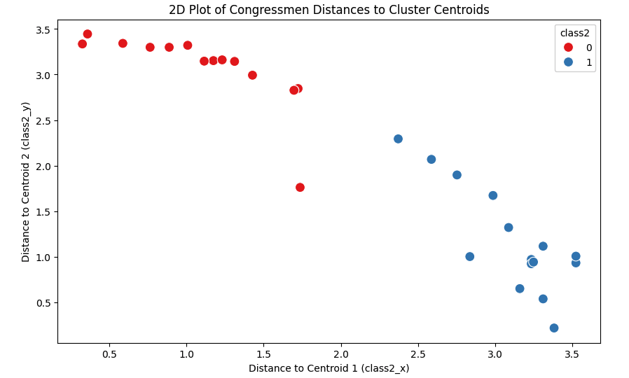
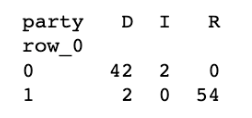
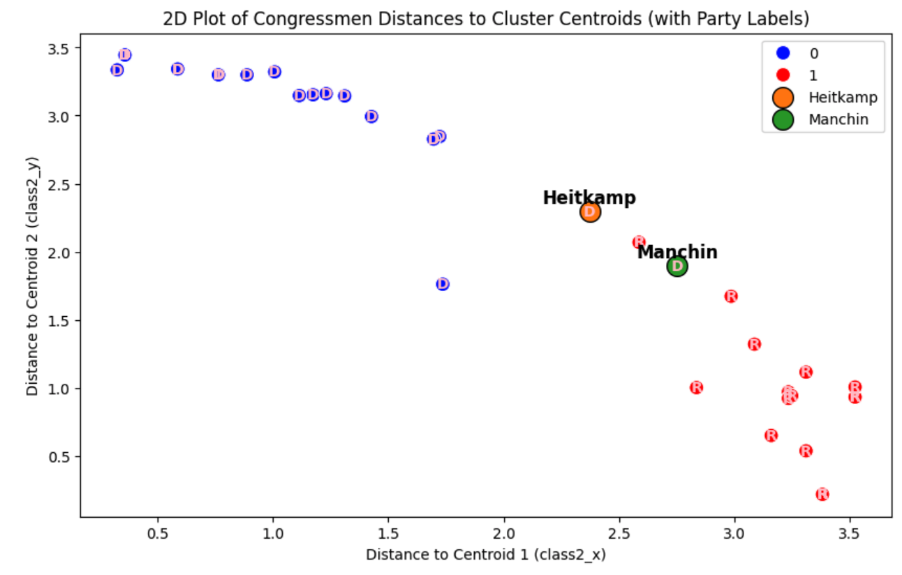
发现按2类划分的时候，确实基本符合只有民主党和共和党的两个大党对应的两种风格，但检查交叉矩阵，发现有些民主党成员被划分到了共和党那一类中，疑似“卧底”，可以打印出来看看是谁

We observe that when dividing into 2 clusters, the results generally align with the two major political parties, Democrats and Republicans, each corresponding to a distinct style. However, after inspecting the confusion matrix, we find that some Democratic members have been grouped into the Republican cluster, raising suspicion that they might be "apostate" members. We can print their names to see who they are.

apostate = votes[(votes['party'] == 'D') & (votes['class2'] == 1)]
apostate

DBSCAN算法 DBSCAN Clustering

在K-means算法中，需要自己指定K值，也就是确定最终要得到多少个类别，那么，能不能让算法自 动决定数据集划分成多少个类别呢?那些不规则的簇该怎么解决呢?下面介绍的DBSCAN算法就能在一 定程度上解决这些问题。

In the K-means algorithm, you need to specify the value of K yourself, meaning you must determine how many clusters you want to end up with. But is it possible for the algorithm to automatically decide how many clusters the dataset should be divided into? And how do we handle irregularly shaped clusters? The DBSCAN algorithm, introduced below, can address these issues to some extent.

在介绍建模流程之前，需要了解它的一些基本概念，略微比K-means算法复杂。

(1)ε-邻域:给定对象半径r内的邻域。K-means算法是基于距离计算的，但是在DBSCAN中，最 核心的参数是半径，会对结果产生较大影响。

(2)核心点:如果对象的ε-邻域至少包含一定数目的数据点，则称该数据点为核心对象，说明这个数据点周围比较密集。

(3)边界点:边界点不是核心点，但落在某个核心点的邻域内，也就是在数据集中的边界位置。

(4)噪声点:既不是核心点，也不是边界点的其他数据点，也就是数据点落单了。

Before introducing the modeling process, it's important to understand some basic concepts, which are slightly more complex than those in the K-means algorithm.

(1)ε-neighborhood: The neighborhood within a given radius (r) of an object. While the K-means algorithm is based on distance calculations, in DBSCAN, the most critical parameter is the radius, which greatly impacts the results.

(2)Core point: If the ε-neighborhood of an object contains at least a certain number of data points, then that data point is called a core object, indicating that the area around this point is relatively dense.

(3)Border point: A border point is not a core point, but it lies within the neighborhood of a core point, meaning it is located at the edge of a cluster in the dataset.

(4)Noise point: A data point that is neither a core point nor a border point, meaning it is isolated from other data points.

步骤 Steps

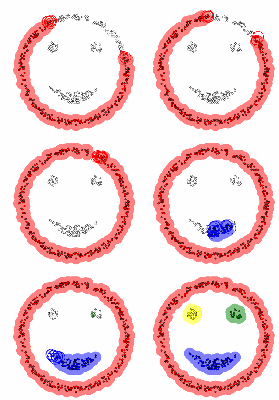
1. 参数设定：设定两个重要参数：

    ε（eps）：定义领域的半径，即在该半径范围内的点被视为邻居。

    MinPts：在 ε 半径内至少需要包含的点数目，才能将该点视为“核心点”。

2. 遍历每个数据点：

    如果某个点已经被访问过，跳过它。

    如果该点没有被访问过，则标记为已访问。

3. 划分点以及核心：

    如果某个数据点的邻居数目不小于 MinPts，则该点被标记为“核心点”，如果该点是从别的类的核心过来的，划入上个核心的类中，否则创建一个新聚类。

    如果邻居数小于 MinPts，如果该点是从别的类的核心过来的，划入上个核心的类中，否则该点被标记为“噪声点”，但它可能会在后续步骤中被重新分配到某个类里。

4. 扩展聚类：

    对每个核心点，将其邻居加入到同一个聚类中。

    对新加入聚类的邻居点，如果它们也是核心点，继续向外扩展，直到无法再扩展为止。

5. 处理边界点：

    如果一个点是某个核心点的邻居，但它本身不满足核心点的条件（邻居数 < MinPts），则该点被标记为边界点，并归属于该核心点的聚类。

6. 算法终止：重复上述过程，直到所有点都被处理为止。

1. Parameter Setup: Set two important parameters:

    ε (eps): Defines the radius of the neighborhood, meaning points within this radius are considered neighbors.

    MinPts: The minimum number of points required within the ε-radius for a point to be considered a "core point."

2. Traverse each data point:

    If a point has already been visited, skip it.

    If the point has not been visited, mark it as visited.

3. Classify points and identify cores:

    If the number of neighbors of a data point is greater than or equal to MinPts, the point is marked as a "core point." If the point comes from the core of another cluster, it is assigned to that core’s cluster; otherwise, a new cluster is created.

    If the number of neighbors is less than MinPts, and the point comes from the core of another cluster, it is assigned to that core’s cluster. Otherwise, the point is marked as a "noise point." However, it may be reassigned to a cluster in subsequent steps.

4. Expand the cluster:

    For each core point, add its neighbors to the same cluster.

    If the newly added neighbors are also core points, continue expanding outward until no further expansion is possible.

5. Handle border points:

    If a point is a neighbor of a core point but does not meet the conditions to be a core point itself (i.e., its number of neighbors < MinPts), it is marked as a border point and assigned to the cluster of the core point.

6. Algorithm termination: Repeat the above process until all points have been processed.

相关参数 Relevant Parameters

1. ε（eps）：邻域半径

    影响：ε 定义了一个点的邻域范围，决定哪些点被视为是彼此的邻居。

    ε 太小：每个点的邻域包含的点太少，可能导致形成很多小的、分散的簇，甚至所有点都可能被标记为噪声点。

    ε 太大：邻域范围过大，可能导致不同密度的簇被合并成一个大簇，无法区分出不同的聚类结构。

2. MinPts：最小邻居点数

    影响：MinPts 决定一个点是否能成为“核心点”，即它邻域中至少要有 MinPts 个点（包括自己）才能形成聚类。

    MinPts 太小：容易将密度较低的区域也标记为聚类，导致噪声点被错误地包含在聚类中。

    MinPts 太大：要求每个核心点周围必须有很多点，可能导致一些稀疏区域的点（本应属于某个簇）被标记为噪声。

1. ε (eps): Neighborhood radius

    Impact: ε defines the neighborhood range of a point, determining which points are considered neighbors of each other.

    ε too small: If ε is too small, the neighborhood of each point will contain very few points, which may lead to many small and scattered clusters, or even all points being marked as noise.

    ε too large: If ε is too large, the neighborhood range becomes too broad, which may cause clusters of different densities to be merged into one large cluster, making it impossible to distinguish different clustering structures.

2. MinPts: Minimum number of neighboring points

    Impact: MinPts determines whether a point can become a "core point." A point must have at least MinPts points (including itself) in its neighborhood to form a cluster.

    MinPts too small: If MinPts is too small, areas with lower density may also be marked as clusters, leading to noise points being incorrectly included in clusters.

    MinPts too large: If MinPts is too large, each core point must have many points around it, which may cause points in sparse regions (that should belong to a cluster) to be marked as noise.

代码实例  Code Example

有一份NBA球员的数据如下

There is a dataset containing NBA players' statistics.

import pandas as pd
from sklearn.model_selection import train_test_split
from sklearn.preprocessing import LabelEncoder, StandardScaler

nba = pd.read_csv("./nba_2013.csv")
nba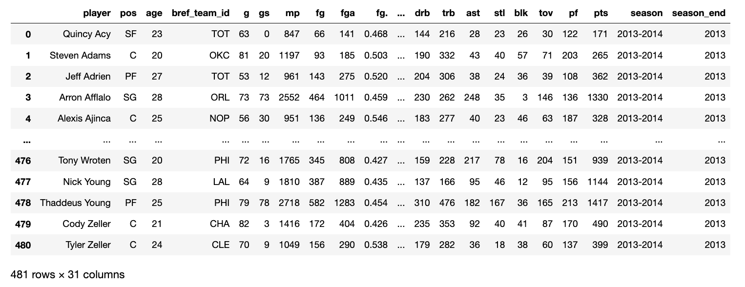

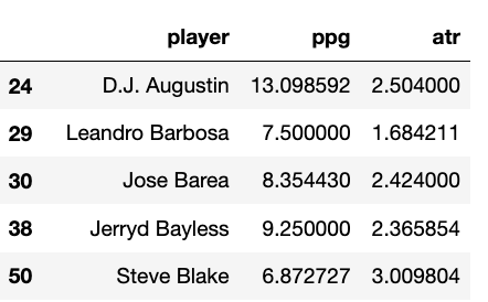
我们取后卫的数据，并计算两个维度（场均分=总分/场次，效率=助攻数/失误数量）来进行分类，并画出分布图

We extract the data for guards and calculate two metrics (points per game = total points / games played, efficiency = assists / turnovers) for classification, and plot the distribution.

# two dimensions
point_guards = nba[nba['pos'] == 'PG'].copy()
point_guards['ppg'] = point_guards['pts'] / point_guards['g']
point_guards = point_guards[point_guards['tov'] != 0]
point_guards['atr'] = point_guards['ast'] / point_guards['tov']
point_guards[['player', 'ppg', 'atr']]

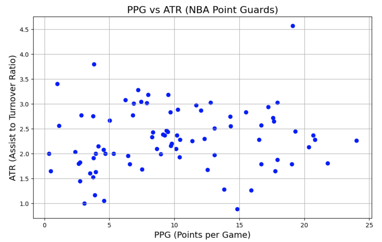
定义不同的eps和min_samples组合，并使用DBSCAN进行分类得到对应结果

We define different combinations of eps and min_samples, and use DBSCAN for classification to obtain the corresponding results.

# DBSCAN可视化 (4x4子图，枚举不同的eps和min_samples)
import matplotlib.pyplot as plt
from sklearn.cluster import DBSCAN
from sklearn.preprocessing import StandardScaler
import numpy as np

# 假设 point_guards 是一个包含数据的 DataFrame
# 提取数据 (ppg: 场均分, atr: 助攻失误比)
X = point_guards[['ppg', 'atr']]
# 标准化数据
scaler = StandardScaler()
X_scaled = scaler.fit_transform(X)
# 定义不同的eps和min_samples组合
eps_values = [0.2, 0.3, 0.4, 0.5]
min_samples_values = [3, 4, 5, 6]
# 创建子图 (4*4)
fig, axes = plt.subplots(4, 4, figsize=(20, 20))
# 遍历每个eps和min_samples的组合
for i, eps in enumerate(eps_values):
    for j, min_samples in enumerate(min_samples_values):
        # 在第(i, j)个子图中绘制
        ax = axes[i, j]
        # 使用DBSCAN进行聚类
        dbscan = DBSCAN(eps=eps, min_samples=min_samples)
        clusters = dbscan.fit_predict(X_scaled)
        # 绘制散点图，按不同簇显示不同颜色
        unique_labels = np.unique(clusters)
        for label in unique_labels:
            if label == -1:
                # 标记噪声点
                color = 'k'
                label_name = "Noise"
            else:
                color = plt.cm.Spectral(float(label) / len(unique_labels))
                label_name = f"Cluster {label}"
            ax.scatter(X_scaled[clusters == label, 0], X_scaled[clusters == label, 1], 
                       label=label_name, c=[color], s=50)
        # 添加子图标题和轴标签
        ax.set_title(f'eps={eps}, min_samples={min_samples}', fontsize=12)
        ax.set_xlabel('Standardized PPG', fontsize=10)
        ax.set_ylabel('Standardized ATR', fontsize=10)
        # 显示图例
        ax.legend()
# 调整子图布局
plt.tight_layout()
# 显示整张图
plt.show()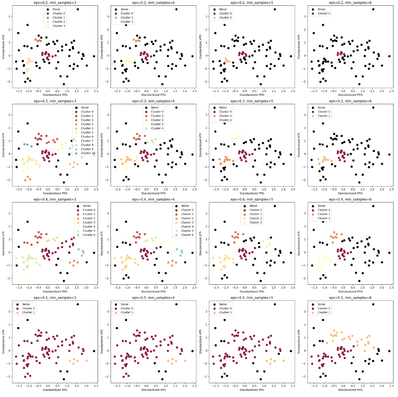

总结 Summary

本章介绍了两种最常用的聚类算法——K-means和DBSCAN，其工作原理不同，在处理不同效果时也 有一定差别。在使用时，需要先分析数据可能的分布形状，再选择合适的算法，因为它们在处理不同类 型数据时各有优缺点。

This chapter introduced two of the most commonly used clustering algorithms—K-means and DBSCAN. They operate based on different principles and show varying performance under different conditions. When using them, it's important to first analyze the possible distribution shapes of the data and then choose the appropriate algorithm, as each has its own advantages and disadvantages when handling different types of data.

比较麻烦就是选择参数，无论是K值还是半径都是令人十分头疼的问题，需要针对具体问题，选择可 行的评估方法后进行实验对比分析。

The most troublesome part is selecting the parameters, whether it's the value of K or the radius, which can be quite challenging. It requires choosing a feasible evaluation method based on the specific problem and then conducting experimental comparisons and analysis.

不同的聚类算法得到的结果差异会比较大，即便同一种算法，使用不同参数时的结果也是完全不 同。由于本身的无监督性，使得结果评估也成为一个难题，最终可以得到每个样本点各自的划分，但是效果怎么样却很难解释，所以聚类还存在如何自圆其说的一个问题。

The results from different clustering algorithms can vary significantly, and even with the same algorithm, using different parameters can yield completely different results. Due to the unsupervised nature of clustering, evaluating the results becomes a challenge. Although we can obtain each sample's cluster assignment, it is often difficult to explain how well the clustering worked, leading to the issue of justifying the results.

一般情况下，当有数据标签的时候，还是老老实实地用有监督算法，实在没办法再选聚类。

In general, when data labels are available, it is better to stick with supervised algorithms. Clustering should only be considered when no other method is feasible.