初识神经网络 First Encounter with Neural Networks

背景 Background

本节介绍当下机器学习中非常火爆的算法——神经网络，深度学习的崛起更是让神经网络名声大振，在计算机视觉、自然语言处理和语音识别领域都有杰出的表现。

This section introduces a highly popular algorithm in contemporary machine learning—neural networks. The rise of deep learning has further boosted the reputation of neural networks, showcasing remarkable performance in fields such as computer vision, natural language processing, and speech recognition.

神经网络其实是一个很古老的算法，那么，为什么现在才流行起来呢?一方面，神经网络算法需要 大量的训练数据，现在正是大数据时代，可谓是应景而生。另一方面，不同于其他算法只需求解出几个 参数就能完成建模任务，神经网络内部需要千万级别的参数来支撑，所以它面临的最大的问题就是计算 的效率，想求解出这么多参数不是一件容易的事。随着计算能力的大幅度提升，这才使得神经网络重回舞台中央。

Neural networks are actually a very old algorithm, so why have they become popular only now? On one hand, neural networks require a large amount of training data, and we are now in the era of big data, making it a fitting time for their resurgence. On the other hand, unlike other algorithms that can accomplish modeling tasks by solving just a few parameters, neural networks need to be supported by millions of parameters internally. Thus, the biggest challenge they face is computational efficiency—solving such a vast number of parameters is not an easy task. With the significant advancements in computational power, neural networks have returned to center stage.

数据计算的过程通常都涉及与矩阵相关的计算，由于神经网络要处理的计算量非常大，仅靠CPU迭 代起来会很慢，一般会使用GPU来加快计算速度，GPU的处理速度比CPU至少快100倍。

The process of data computation often involves matrix-related calculations. Given the enormous amount of computations that neural networks have to handle, relying solely on a CPU would make iteration very slow. Typically, GPUs are used to accelerate the computation, as they are at least 100 times faster than CPUs.

神经网络很像一个黑盒子，只要把数据交给它，并且告诉它最终要想达到的目标，整个网络就会开 始学习过程，由于涉及参数过多，所以很难解释神经网络在内部究竟做了什么。在之前的机器学习任务中，特征工程是一个核心模块，在算法执行前，通常需要替它选出最好的且最有价 值的特征，这一步通常也是最难的，因为这个过程似乎是人工去一步步解决问题，机器只是完成求解计 算，这与人工智能看起来还有些距离。但在神经网络算法中，终于可以看到些人工智能的影子，只需把 完整的数据交给网络，它会自己学习哪些特征是有用的，该怎么利用和组合特征，最终它会给我们交上 一份答卷，所以神经网络才是现阶段与人工智能最接轨的算法。

Neural networks resemble a black box: once data is fed into the network and the desired objective is specified, the entire network begins the learning process. Due to the large number of parameters involved, it is difficult to explain exactly what happens inside the neural network. In previous machine learning tasks, feature engineering was a core module. Before executing an algorithm, it was usually necessary to manually select the best and most valuable features for the task. This step was often the hardest, because the process seemed to involve humans solving problems step by step, while the machine only handled the computations. This approach seemed somewhat distant from artificial intelligence. However, with neural networks, we can finally see some traces of AI—just by feeding the complete data into the network, it will learn by itself which features are useful and how to utilize and combine those features. In the end, the network will provide us with an answer sheet, which makes neural networks the algorithm most aligned with AI at this stage.

基本上所有机器学习问题都能用神经网络来解决，但其中也会存在一些影响因素，那就 是过拟合问题比较严重，所以还是那句话——能用逻辑回归解决的问题根本没有必要拿到神经网络中。 神经网络的效果虽好，但是效率却不那么尽如人意，训练网络需要等待的时间也十分漫长，毕竟要求解几千万个参数，短时间内肯定完不成，所以还是需要看具体任务的要求来选择不同的算法。

Almost all machine learning problems can be solved using neural networks, but there are influencing factors, such as the issue of overfitting, which can be quite serious. Hence, as the saying goes: “if a problem can be solved with logistic regression, there’s no need to bring it to a neural network.” While neural networks deliver good results, their efficiency is less than ideal. Training a network requires a long waiting time—after all, solving tens of millions of parameters cannot be completed in a short time. So ultimately, the choice of algorithm should depend on the specific requirements of the task.

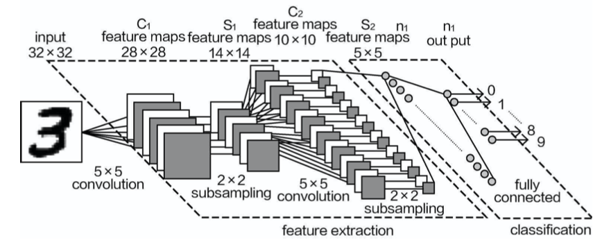
神经网络模块 Neural Network Modules

如果直接看整个神经网络，可能会觉得有些复杂，先挑一些基础模块的原理及其工作流程进行讲解

At first glance, an entire neural network might seem a bit complex. Let’s start by explaining some basic modules, their principles, and workflows.

得分函数 Score Function

下面准备完成图像分类的任务，如何才能确定一个输入属于哪个类别呢?需要神经网络最终输出一个结果(例如一个分值)，以评估它属于各个类别的可能性，假设输入数据是32×32×3，一共就有3072个像素点，每一个都会对最终结果产生影响，但其各自的影 响应当是不同的，例如猫的耳朵、眼睛部位会对最终结果是猫产生积极的影响，而一些背景因素可能会 对最终结果产生负面的影响。这就需要分别对每个像素点加以计算，此时就需要3072个权重参数(和像 素点个数一一对应)来控制其影响大小，如图

Now, we’re preparing to complete an image classification task. How do we determine which category an input belongs to? We need the neural network to output a result (for example, a score) that evaluates the likelihood of the input belonging to each category. Suppose the input data is 32×32×3, which means there are 3,072 pixels in total. Each of these pixels will influence the final result, but their individual influences should differ. For example, a cat’s ears and eyes will positively influence the final result of it being classified as a cat, while some background elements may have negative effects on the final result. This requires calculating the influence of each pixel individually. At this point, 3,072 weight parameters (corresponding one-to-one with the pixels) are needed to control the magnitude of each pixel’s influence, as shown in the diagram.

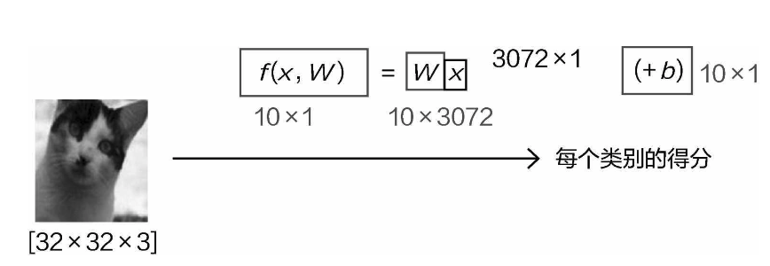
如果只想得到当前的输入属于某一个特定类别的得分，只需要一组权重参数(1×3072)就足够了。 那么，如果想做的是十分类问题呢?此时就需要十组权重参数，例如还有狗、船、飞机等类别，每组参 数用于控制当前类别下每个像素点对结果作用的大小。

If you only want to get the score for the input belonging to one specific category, one set of weight parameters (1×3,072) is enough. But what if you’re working on a ten-class classification problem? In that case, you would need ten sets of weight parameters — for example, for categories like dog, ship, airplane, etc. Each set of parameters would control the extent to which each pixel influences the result for the current category.

不要忽略偏置参数b，它相当于微调得到的结果，让输出能够更精确。所以最终结果主要由权重参数w来控制，偏置参数b只是进行微调。如果是十分类任务，各自类别都需要进行微调，也就是需要10个 偏置参数。

Don’t overlook the bias parameter b. It essentially fine-tunes the result, making the output more precise. So, the final result is primarily controlled by the weight parameters w, with the bias parameter b just making small adjustments. In a ten-class classification task, each category requires its own fine-tuning, meaning ten bias parameters are needed.

接下来通过一个实际的例子看一下得分函数的计算流程：

Next, let’s look at the process of calculating the score function through a practical example:

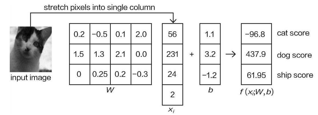
输入还是这张猫的图像，简单起见就做一个三分类任务，最终得到当前输入属于每一个类别的得分值。观察可以发现，权重参数和像素点之间的关系是一一对应的，有些权重参数比较大，有些比较小， 并且有正有负，这就是表示模型认为该像素点在当前类别的重要程度，如果权重参数为正且比较大，就意味着这个像素点很关键，对结果是当前类别起到促进作用。

The input is still an image of a cat, and for simplicity, we’ll work on a three-class classification task, ultimately obtaining the scores for the current input belonging to each category. As you can see, the relationship between the weight parameters and the pixel points is one-to-one. Some weight parameters are large, some are small, and some are positive while others are negative. This indicates how important the model considers each pixel to be for the current category. If a weight parameter is both positive and large, it means that the pixel is critical and promotes the result being classified as the current category.

那么怎么确定权重和偏置参数的数值呢?实际上需要神经网络通过迭代计算逐步更新，这与梯度下 降中的参数更新道理是一样的，首先随机初始化一个值，然后不断进行修正即可。

So, how do we determine the values of the weight and bias parameters? In fact, the neural network needs to iteratively update them, which follows the same principle as parameter updates in gradient descent. First, a random value is initialized, and then it is continuously adjusted.

从最终分类的得分结果上看，原始输入是一只小猫，但是模型却认为它属于猫这个类别的得分只有 −96.8，而属于其他类别的得分反而较高。这显然是有问题的，本质原因就是当前这组权重参数效果并不 好，需要调整找到更好的参数组合。

From the final classification score result, the original input is an image of a cat, but the model thinks the score for it belonging to the cat category is only −96.8, while the scores for other categories are relatively higher. Clearly, this is problematic. The fundamental reason is that the current set of weight parameters is not effective, and better parameters need to be found through adjustment.

损失函数 Loss Function

由于预测结果和真实情况的差异比较大，需要用一个具体的指标来评估当前模型效果的好坏，并且要用一个具体数值分辨好坏的程度，这就需要用损失函数来计算。

Due to the significant difference between the predicted results and the actual situation, we need a specific metric to evaluate how good or bad the current model is. Furthermore, we need a concrete numerical value to distinguish the degree of accuracy or error. This is where the loss function comes into play.

损失函数的值越小，表示模型的预测结果越接近真实值。通过反向传播算法，神经网络会根据损失函数的梯度来调整网络中的参数，使得下一次的预测更加准确。

The smaller the value of the loss function, the closer the model’s prediction is to the true value. Through the backpropagation algorithm, the neural network adjusts the parameters within the network based on the gradient of the loss function, making the next prediction more accurate.

在损失函数中，还加入了正则化惩罚项，这一步也是必须的，因为神经网络实在太容易过拟合。

Additionally, a regularization penalty is included in the loss function. This step is necessary because neural networks are highly prone to overfitting.

反向传播 Backpropagation

现在已经完成了从输入数据到计算损失的过程，通常把这部分叫作前向传播。但是网络模型最终的结果完全是由其中的权重与偏置参数来决定的， 所以神经网络中最核心的任务就是找到最合适的参数。

Now that we have completed the process from input data to calculating the loss, this part is usually referred to as forward propagation. However, the final result of the network model is entirely determined by its weight and bias parameters, so the core task in a neural network is to find the most appropriate parameters.

前面已经讲解过梯度下降方法，很多机器学习算法都是用这种优化的思想来迭代求解，神经网络也是如此。当确定损失函数之后，就转化成了下山问题。但是神经网络是层次结构，不能一次梯度下降就得到所有参数更新的方向，需要逐层完成更新参数工作。

We’ve already discussed the gradient descent method earlier. Many machine learning algorithms use this optimization idea to iteratively solve problems, and neural networks are no exception. Once the loss function is determined, it essentially becomes a descent problem. However, since a neural network has a hierarchical structure, we can’t update all parameters in a single gradient descent step; instead, parameters must be updated layer by layer.

由于网络层次的特性，在计算梯度的时候，需要遵循链式法则，也就是逐层计算梯度，并且梯度是可以传递的，例如以下函数：

Due to the layered nature of the network, we need to follow the chain rule when calculating gradients, which means calculating the gradient layer by layer, and the gradients can be propagated. For example, consider the following functions:

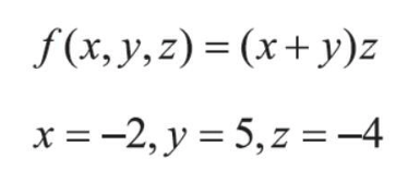
既然要对参数进行更新，可以看一看不同的参数对模型的损失做了什么贡献。如果一个参数使得模 型的损失增大，那就要削减它;如果一个参数能使得模型的损失减小，那就增大其作用。上述例子中， 就是把x,y,z分别看成影响最终结果的3个因子，现在要求它们对结果的影响有多大:

Since we want to update the parameters, we can look at how each parameter contributes to the model’s loss. If a parameter increases the model's loss, we should reduce it; if a parameter decreases the loss, we should increase its influence. In the example above, we treat x, y, and z as three factors influencing the final result, and we need to determine how much they contribute to the result:

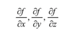
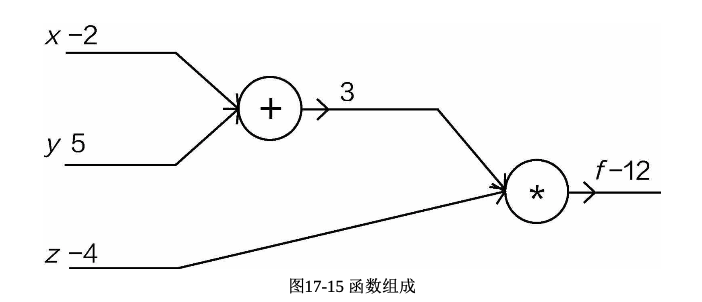
通过计算可以看出，当计算x和y对结果的贡献时，不能直接进行计算，而是间接计算q=(x+y)对结果的贡 献，再分别计算x和y对q=(x+y)的贡献。在神经网络中，并不是所有参数的梯度都能一步计算出来，要按照其位置顺序，一步步进行传递计算，这就是反向传播

Through the calculations, we can see that when calculating the contributions of x and y to the result, we cannot compute them directly. Instead, we first calculate the contribution of q = (x + y) to the result, and then calculate the contributions of x and y to q = (x + y), respectively. In a neural network, not all parameter gradients can be computed in one step; rather, they need to be propagated and calculated step by step in order of their position. This process is backpropagation.

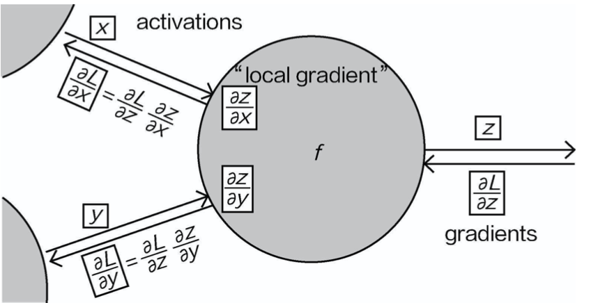
从整体上来看，优化方法依旧是梯度下降法，只不过是逐层进行的。反向传播的计算求导相对比较复杂，建议大家先了解其工作原理，具体计算交给计算机和框架完成。

From an overall perspective, the optimization method is still gradient descent, but it is performed layer by layer. Backpropagation's gradient calculation is relatively complex, so it is recommended to first understand the working principles, and leave the specific calculations to computers and frameworks.

神经网络架构 Neural Network Architecture

接下来要把它们组合成一个完整的神经网络，从整体上看神经网络到底做了什么。

Next, we will combine the components into a complete neural network to see what a neural network does from a holistic perspective.

整体框架 Overall Framework

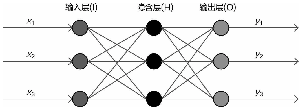
神经网络整体架构如图1。可以看出，神经网络是一个层次结构，包括输入层、隐藏层和输出层。

The overall architecture of a neural network is shown in Figure 1. As you can see, a neural network has a layered structure, including an input layer, hidden layers, and an output layer.

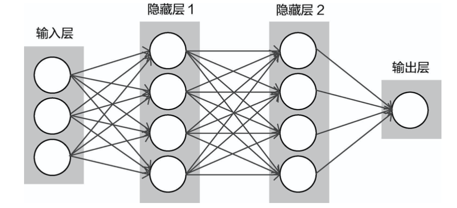
(1)输入层。图17-17的输入层中画了3个圆，通常叫作3个神经元，即输入数据由3个特征或3个像 素点组成。

(1)Input Layer: In the input layer of Figure 17-17, there are 3 circles drawn, which are often referred to as 3 neurons. This means that the input data consists of 3 features or 3 pixels.

(2)隐藏层1。输入数据与隐藏层1连接在一起。神经网络的目标就是寻找让计算机能更好理解的特 征，这里面画了4个圆(4个神经元)，可以当作通过对特征进行某种变换将原始3个特征转换成4个特征(实际情况下，数据特征和隐层特征都是比较大的)

隐藏层的4个特征表示什么意思呢?这个很难 解释，神经网络会按照某种线性组合关系将所有特征重新进行组合，之前看到的权重参数矩阵中有正有 负，有大有小，就意味着对特征进行何种组合方式。神经网络是黑盒子的原因也在于此，很难解释其中 过程，只需关注其结果即可。

(2)Hidden Layer 1: The input data is connected to the first hidden layer. The goal of the neural network is to find features that the computer can better understand. There are 4 circles (representing 4 neurons) drawn here, which can be thought of as transforming the original 3 features into 4 features through some kind of transformation (in practice, both the data features and the hidden layer features are much larger). What do the 4 features in the hidden layer represent? This is hard to explain. The neural network recombines all the features according to some kind of linear combination. In the weight parameter matrix we saw earlier, some weights are positive, some are negative, some are large, and some are small, indicating how the features are combined. This is also one of the reasons neural networks are considered black boxes—it’s difficult to explain the process, so we focus on the results.

(3)隐藏层2。在隐藏层1中已经对特征进行了组合变换，此时隐藏层2的输入就是隐藏层1变换后的 结果，相当于之前已经进行了某种特征变换，但是还不够强大，可以继续对特征做变换处理，神经网络的强大之处就在于此。如果只有一层神经网络，与之前介绍的逻辑回归差不多，但是一旦有多层层次结 构，整体网络的效果就会更强大。

(3)Hidden Layer 2: In Hidden Layer 1, the features have already been recombined and transformed. At this point, the input to Hidden Layer 2 is the result of the transformation in Hidden Layer 1. This is like applying a feature transformation, but it’s not yet strong enough, so another transformation is performed. This is the strength of neural networks—if there was only one layer, it would be similar to the logistic regression introduced earlier. However, once there is a multi-layer structure, the performance of the entire network becomes much more powerful.

(4)输出层。最终还是要得到结果的，就看要做的任务是分类还是回归，选择合适的输出结果和损 失函数即可，这与传统机器学习算法一致。

(4)Output Layer: Finally, we still need to obtain a result. Whether the task is classification or regression, we select the appropriate output result and loss function, which is consistent with traditional machine learning algorithms.

神经网络中层和层之间都是全连接的操作，也就是隐层中每一个神经元(其中一个特征)都与前面 所有神经元连接在一起，这也是神经网络的基本特性。

In a neural network, each layer is fully connected to the next, meaning that every neuron (feature) in a hidden layer is connected to all the neurons in the previous layer. This is a fundamental characteristic of neural networks.

神经元的作用 The Role of Neurons

概述神经网络的整体架构之后，最值得关注的就是特征转换中的神经元，可以将它理解成转换特征后的维度。

After summarizing the overall architecture of a neural network, the most important aspect to focus on is the neurons involved in feature transformation, which can be understood as the dimensions after the feature transformation.

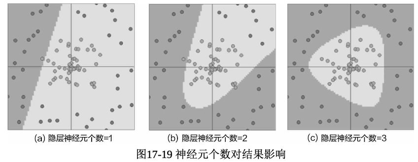
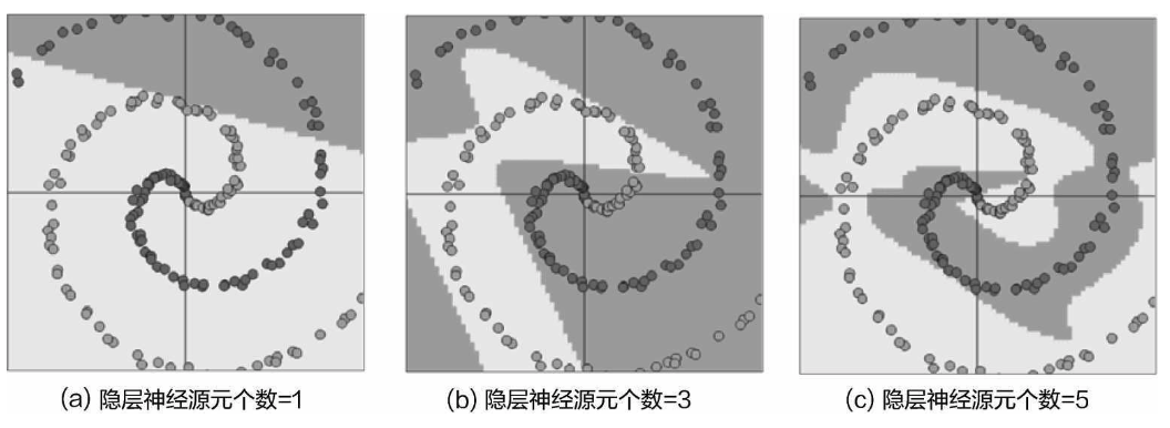
神经元的数量可以自己设计，那么 它会对结果产生多大影响呢?下面看一组对比实验。选择相同的数据集，在网络模型中，只改变隐藏层 神经元个数，得到的结果如图

The number of neurons can be designed manually. So, how much impact does it have on the result? Let’s look at a comparison experiment. Using the same dataset, we only change the number of neurons in the hidden layer of the network model. The results are shown in the figure.

��

当隐藏层神经元数量增大的时候，神经网络可以利用的数据信息就更多，分类效果自然会提高，那么，是不是神经元的数量越多越好呢?在设计神经网络时，不能只考虑最终模型的表现效果，还要考虑计算的可行性与模型的过拟合风险。

When the number of neurons in the hidden layer increases, the neural network can utilize more information from the data, naturally improving the classification performance. But does this mean that the more neurons, the better? When designing a neural network, we cannot only consider the final model performance but must also take into account the feasibility of computation and the risk of overfitting.

正则化 Regularization

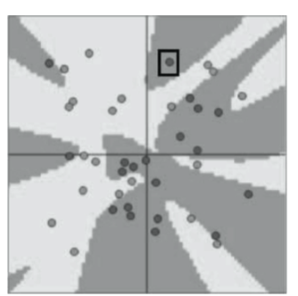
神经网络效果虽然强大，但是过拟合风险实在是高，由于其参数过多，所以必须进行正则化处理， 否则即便在训练集上效果再高，也很难应用到实际中。

Although neural networks are powerful, they carry a high risk of overfitting. Due to the large number of parameters, regularization is essential. Otherwise, even if the performance on the training set is excellent, it will be difficult to apply the model in real-world scenarios.

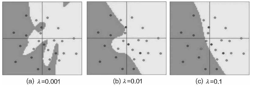
最常见的正则化惩罚是L2范数，即对权重参数中所有元素求平方和，显然，只与权重 有关系，而和输入数据本身无关，只惩罚权重。

在计算正则化惩罚时，还需引入惩罚力度，也就是λ，表示希望对权重参数惩罚的大小，选择不同的惩罚力度在神经网络中的效果差异还是比较大的。

The most common regularization penalty is the L2 norm, which calculates the sum of the squares of all elements in the weight parameters. Clearly, this is only related to the weights and not to the input data itself—it penalizes only the weights.

When calculating the regularization penalty, a penalty strength (denoted by λ) must also be introduced, which represents how strongly the weights should be penalized. Different penalty strengths can have a significant impact on the performance of the neural network.

当惩罚力度较大时，模型的边界就会变得比较平稳，虽然有些数据点并没有完全划分正确，但是这 样的模型实际应用效果还是不错的，过拟合风险较低。

When the penalty strength is high, the model’s decision boundaries become smoother. Although some data points may not be classified correctly, such a model still performs well in practice and has a lower risk of overfitting.

通过上述对比可以发现，不同的惩罚力度得到的结果完全不同，那么如何进行选择呢?还是一个调 参的问题，但是，通常情况下，宁可选择图(c)中的模型，也不选择图(a)中的模型，因为 其泛化能力更强，效果稍微差一点还可以忍受，但是完全过拟合就没用了。

By comparing the results, we can see that different penalty strengths lead to completely different outcomes. So, how should we choose? It’s a matter of hyperparameter tuning, but in most cases, it’s better to choose a model like the one shown in figure (c) rather than figure (a) because it has stronger generalization ability. Slightly worse performance can be tolerated, but complete overfitting renders the model useless.

激活函数 Activation Function

在神经网络的整体架构中，将数据输入后，一层层对特征进行变换，最后通过损失函数评估当前的 效果，这就是前向传播。接下来选择合适的优化方法，再反向传播，从后往前走，逐层更新权重参数。

In the overall architecture of a neural network, after inputting the data, the features are transformed layer by layer, and finally, the performance is evaluated using a loss function—this process is called forward propagation. Next, an appropriate optimization method is chosen, and through backpropagation, the network works backward, updating the weight parameters layer by layer.

如果层和层之间都是线性变换，那么，只需要用一组权重参数代表其余所有的乘积就可以了。这样 做显然不行，一方面神经网络要解决的不仅是线性问题，还有非线性问题;另一方面，需要对变换的特 征加以筛选，让有价值的权重特征发挥更大的作用，这就需要激活函数。

If the transformations between layers were purely linear, then one set of weight parameters could represent all the other products. Clearly, this approach would not work. On the one hand, neural networks are designed to solve not only linear problems but also nonlinear ones. On the other hand, it’s necessary to filter the transformed features, allowing valuable weight features to have a greater impact. This is where the activation function comes into play.

代码示例 Code Example

18.2 搭建神经网络进行手写字体识别.pdf

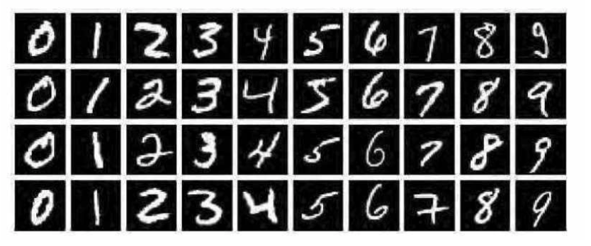
下面向大家介绍经典的手写字体识别数据集—Mnist数据集，如图18-4所示。数据集中包括0~9十个数字，我们要做的就是对图像进行分类，让神经网络能够区分这些手写字体。

Next, we introduce the classic handwritten digit recognition dataset—the MNIST dataset, as shown in Figure 18-4. The dataset includes ten digits from 0 to 9, and our task is to classify the images so that the neural network can distinguish between these handwritten digits.

选择这份数据集的原因是其规模较小(28×28×1)，用笔记本电脑也能执行它，非常适合学习。通常 情况下，数据大小(对图像数据来说，主要是长、宽、大、小)决定模型训练的时间，对于较大的数据 集(例如224×224×3)，即便网络模型简化，还是非常慢。对于没有GPU的初学者来说，在图像处理任务 中，Mnist数据集就是主要练习对象。

The reason for choosing this dataset is its relatively small size (28×28×1), which allows it to be executed even on a laptop, making it very suitable for learning. Generally, the size of the data (for image data, this refers to the length, width, and the overall size) determines the training time of the model. For larger datasets (e.g., 224×224×3), training is still very slow, even if the network model is simplified. For beginners without a GPU, the MNIST dataset is the main practice target for image processing tasks.

下载数据，里面已经分好了训练集和测试集

Download the dataset, which already includes separate training and test sets.

import numpy as np
import os
import tensorflow as tf
# 使用 Keras 的接口加载 MNIST 数据集
(x_train, y_train), (x_test, y_test) = tf.keras.datasets.mnist.load_data()
# 本地目录路径
data_dir = './my_mnist_data/'
if not os.path.exists(data_dir):
    os.makedirs(data_dir)
# 将数据保存为 .npy 文件
np.save(os.path.join(data_dir, 'x_train.npy'), x_train)
np.save(os.path.join(data_dir, 'y_train.npy'), y_train)
np.save(os.path.join(data_dir, 'x_test.npy'), x_test)
np.save(os.path.join(data_dir, 'y_test.npy'), y_test)
print("MNIST 数据集已保存到本地目录！")

搭建神经网络，可构建一层或多层隐藏层，指定神经元个数

Build the neural network, which can consist of one or more hidden layers, and specify the number of neurons.

import tensorflow as tf
from tensorflow.keras import layers, models
import numpy as np
import matplotlib.pyplot as plt

# 1. 加载MNIST数据集 / Load the MNIST dataset
(x_train, y_train), (x_test, y_test) = tf.keras.datasets.mnist.load_data()

# 数据预处理：将图像展平为784维向量，并将像素值归一化到[0, 1]
# Data preprocessing: flatten images to 784-dimensional vectors and normalize pixel values to [0, 1]
x_train = x_train.reshape(-1, 28*28).astype('float32') / 255.0
x_test = x_test.reshape(-1, 28*28).astype('float32') / 255.0

# 2. 构建简单的神经网络模型 / Build a simple neural network model
model = models.Sequential([
    layers.InputLayer(input_shape=(28*28,)),  # 输入层，28x28像素展平为784个输入 / Input layer, 28x28 pixels flattened to 784 inputs
    layers.Dense(64, activation='relu'),     # 隐藏层，64个神经元，激活函数为ReLU / Hidden layer, 64 neurons, activation function is ReLU
    layers.Dense(10, activation='softmax')    # 输出层，10个类别，使用Softmax激活 / Output layer, 10 classes, using Softmax activation
])

# 3. 编译模型，指定损失函数、优化器和评估指标
# Compile the model, specifying the loss function, optimizer, and evaluation metrics
model.compile(optimizer='adam',
              loss='sparse_categorical_crossentropy',
              metrics=['accuracy'])
              
# 4. 训练模型 / Train the model
model.fit(x_train, y_train, epochs=20, batch_size=32)

# 5. 在测试集上评估模型 / Evaluate the model on the test set
test_loss, test_acc = model.evaluate(x_test, y_test)
print(f"测试集准确率: {test_acc:.4f}")  # Test accuracy

# 6. 进行所有测试集的预测 / Make predictions on the entire test set
predictions = model.predict(x_test)
# 将预测结果转换为类别索引 / Convert prediction results to class indices
predicted_labels = np.argmax(predictions, axis=1)

# 7. 找到预测错误的样本 / Find incorrectly predicted samples
incorrect_indices = np.where(predicted_labels != y_test)[0]
# 打印前5个预测错误的样本 / Print the first 5 incorrectly predicted samples
print(f"找到{len(incorrect_indices)}个预测错误的样本。")  # Found {len(incorrect_indices)} incorrectly predicted samples.

# 8. 可视化前几个预测错误的样本 / Visualize the first few incorrectly predicted samples
num_to_display = 5
plt.figure(figsize=(10, 5))
for i, idx in enumerate(incorrect_indices[:num_to_display]):
    plt.subplot(1, num_to_display, i + 1)
    plt.imshow(x_test[idx].reshape(28, 28), cmap='gray')
    plt.title(f"True: {y_test[idx]}, Pred: {predicted_labels[idx]}")
    plt.axis('off')
plt.tight_layout()
plt.show()

查看运行结果

View the results after running.