卷积神经网络原理 Principles of Convolutional Neural Network (CNN)

背景 Background

卷积神经网络是现阶段神经网络中非常火的模型，它在计算机视觉中有着非常不错的效果。不仅如此，卷积神经网络在非图像数据中也有着不错的表现，比如自然语言处理（NLP）、金融数据时序分析、语音处理&情感分析等，可谓在机器 学习领域遍地开花。

Convolutional Neural Networks (CNNs) are currently one of the hottest models in neural networks, and they have shown impressive results in computer vision. Not only that, but CNNs also perform well on non-image data, such as in natural language processing (NLP), financial time series analysis, speech processing, and sentiment analysis. It can be said that they are flourishing across the field of machine learning.

卷积神经网络也是神经网络的一种，本质上来说都是对数据进行特征提取，只不过在图像数据中效 果更好，整体的网络模型架构都是一样的，参数迭代更新也是类似，所以难度就在于卷积上，只需把它 弄懂即可。

Convolutional Neural Networks are a type of neural network, and essentially, they all perform feature extraction on data. However, CNNs tend to work better on image data, though the overall network architecture is the same, and the parameter update process is similar. Therefore, the key challenge lies in understanding convolution, and once you grasp that, the rest follows.

那么，为什么说卷积神经网络在计 算机视觉领域更胜一筹呢?想想之前遇到的问题，神经网络的矩阵计算方式所需参数过于庞大，一方面 使得迭代速度很慢，另一方面过拟合问题比较严重，而卷积神经网络便可以更好地处理这个问题。

So, why are CNNs considered superior in the field of computer vision? Think about the problems encountered before: the matrix computation method in traditional neural networks required an enormous amount of parameters, which not only slowed down the iteration process but also led to serious overfitting issues. Convolutional Neural Networks, on the other hand, can handle this problem more effectively.

卷积操作流程 Convolution Operation Process

接下来就要深入网络细节中，看看卷积究竟做了什么，首先观察一下卷积网络和传统神经网络的不同之处，如图

Next, we will dive into the details of the network to see exactly what convolution does. First, let's observe the differences between a convolutional network and a traditional neural network, as shown in the diagram.

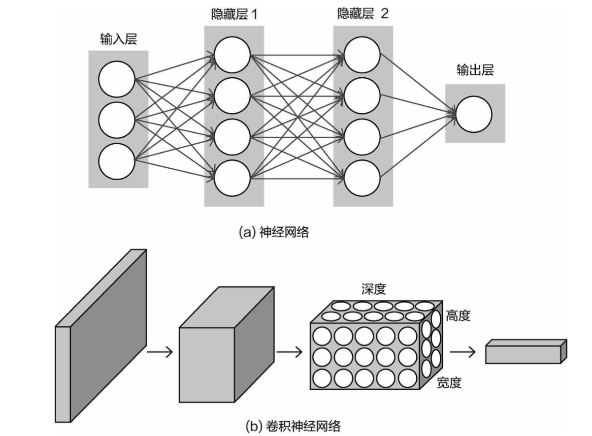
传统的神经网络是一个平面，而卷积网络是一个三维立体的。不难发现，卷积神经网络中多了一个概念——深度。例如图像输入数据h×w×c，其中颜色通道c就是输入的深度。

A traditional neural network operates on a flat plane, whereas a convolutional network operates in three dimensions. It’s easy to notice that Convolutional Neural Networks introduce a new concept—depth. For example, the input image data is represented as h×w×c, where the color channels c correspond to the input depth.

在使用TensorFlow做神经网络的时候，首先将图像数据拉成像素点组成的特征，这样做相 当于输入一行特征数据而非一个原始图像数据，而卷积中要操作的对象是一个整体，所以需要定义深度。如图所示，此时想提取图像中的特征，以前是对每个像素点都 进行变换处理，看起来是独立对待每一个像素点特征。但是图像中的像素点是有一定连续关系的。如果 能把图像按照区域进行划分，再对各个区域进行特征提取应当更合理。

When using TensorFlow to build a neural network, the image data is first flattened into features composed of pixel points. This effectively means that you're inputting a row of feature data rather than the original image data. However, in convolution, the object of operation is the whole image, so depth needs to be defined. As shown in the diagram, when extracting features from the image, the traditional approach was to transform each pixel point individually, treating each pixel feature independently. However, pixels in an image have certain continuous relationships. It would be more reasonable to divide the image into regions and then extract the features from each region.

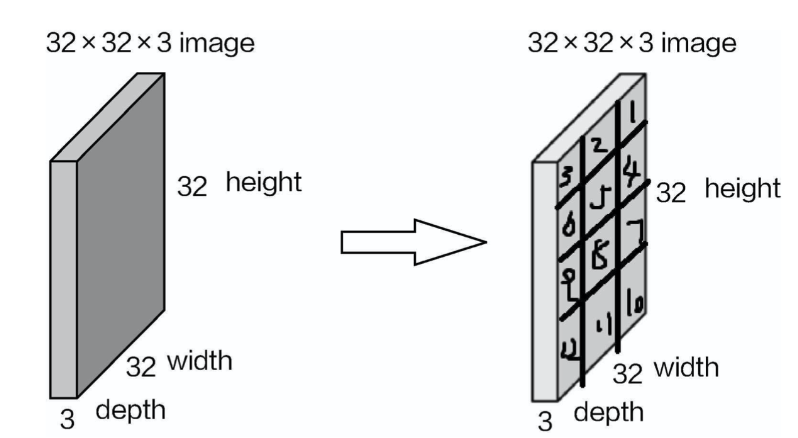
假设把原始数据平均分成多个小块，接下来就要对每一小块进行特征提取，也可以说是从每 一小部分中找出关键特征代表。

Let's assume that we divide the original data into multiple small blocks. Next, we need to extract features from each small block. In other words, we need to find key representative features from each small section.

如何进行体征提取呢?这里需要借助一个帮手，暂时叫它filter，它需要做的就是从其中每一小块区 域选出一个特征值。假设filter的大小是5×5×3，表示它要对输入的每个5×5的小区域都进行特征提取，并 且要在3个颜色通道(RGB)上都进行特征提取再组合起来。

How do we perform feature extraction?For this, we need the help of a tool, which we’ll temporarily call a filter. The filter’s job is to select a feature value from each small region. Suppose the filter size is 5×5×3, meaning it will extract features from each 5×5 small region and perform feature extraction across all three color channels (RGB), then combine them.

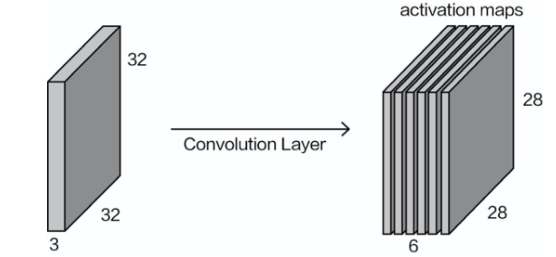
通过助手filter进行特征提取后，就得到图所示的结果，看起来像板子，它们就是特征图，表示特征提取的结果，为什么是两个呢?这里在使用filter进行特征提取的时候，不仅可以用一种特征提取 方法，也就是filter可以有多个，例如在不同的纹理、线条的层面上(只是举例，其实就是不同的权重参数)。

After feature extraction using the helper filter, we get the result shown in the diagram. It looks like plates, which are feature maps representing the results of feature extraction. Why are there two feature maps? When using filters for feature extraction, we can apply more than one extraction method. In other words, there can be multiple filters. For example, they may focus on different textures or lines (this is just a metaphor, as it actually refers to different weight parameters).

例如，在同样的小块区域中，可以通过不同的方法来选择不同层次的特征，最终所有区域特征再组 合成一个整体。在一次特征提取的过程中，如果使用6种不同的filter，那么肯定会得到6张特征图，再把它们堆叠在 一起，就得到了h×w×6的特征输出结果。这其实就是一次卷积操作，如图所示

For example, in the same small area, different methods can be used to select different levels of features. Finally, the features from all regions are combined into one whole. During a single feature extraction process, if we use 6 different filters, we will obtain 6 feature maps. Stacking them together results in a feature output of size h×w×6. This is essentially one convolution operation, as shown in the diagram.

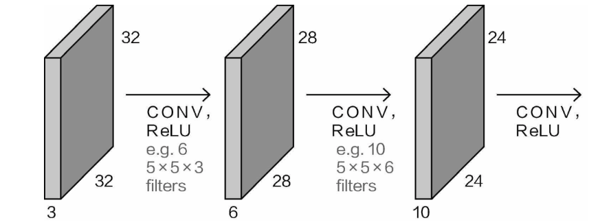
那么是不是只能对输入数据执行卷积操作呢？并不是这样， 我们得到的特征图是28×28×6，感觉它与输入数据的格式差不多。此时第3个维度上，颜色通道数变成特征图个数，所以对特征图继续可以进行卷积操作，相当于在提取出的特征上再进一步提取，得到特征的特征图。

Is convolution only applied to the input data?No, it isn’t. The feature maps we obtain are 28×28×6, which looks similar in format to the input data. The third dimension, which was initially the number of color channels, has now become the number of feature maps. Thus, you can apply convolution operations to the feature maps as well, which is equivalent to extracting features from the extracted features, producing feature maps of features.

卷积的计算方法和相关参数

Convolution Calculation Method and Related Parameters

卷积的计算过程非常简单，当卷积核在输入图像上扫描时，将卷积核与输入图像中对应区域做内积（数值逐个相乘），最后汇总求和，就得到该位置的卷积结果。通过不断移动卷积核，就可算出各个位置的卷积结果。

The convolution process is quite simple. As the convolution filter scans over the input image, it performs a dot product between the filter and the corresponding region of the input image (i.e., multiplying the values element-wise). Finally, the results are summed up to get the convolution result for that position. By continuously moving the filter across the image, you can compute the convolution results for each position.

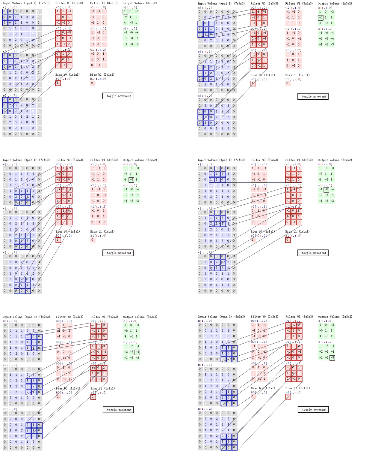
大家可以将输入数据中的数值当作图像中的像素点，但是filter(卷积核)中的数值是什么意思呢？它与神经网络中的权重参数的概念一样，表示对特征进行变换的方法。初始值可以是随机初始化的，然后通过反向传播不断进行更新，最终要求解的就是filter中每个元素的值。

You can think of the numerical values in the input data as the pixel values in an image. But what do the numbers in the filter (convolution kernel) represent? They are conceptually the same as the weight parameters in a neural network and represent the method of transforming the features. The initial values of the filter can be randomly initialized, and then they are updated continuously through backpropagation. Ultimately, the goal is to solve for the values of each element in the filter.

因此，filter(卷积核)就是卷积神经网络中权重参数，最终特征提取的结果主要由它来决定，所以目标就是优化得到最合适的特征提取方式，相当于不断更新其数值。

Therefore, the filter (convolution kernel) in a Convolutional Neural Network (CNN) functions as the weight parameters. The final result of feature extraction is primarily determined by the filter, so the goal is to optimize and find the most appropriate way to extract features, which is achieved by continuously updating its values.

卷积操作比传统神经网络的计算复杂，在设计网络结构过程中，需要给定更多的控制参数：

Convolution operations are more complex than traditional neural network calculations. When designing the network architecture, more control parameters need to be specified:

卷积核Convolution Kernel (Filter)

卷积操作中最关键的就是卷积核，它决定最终特征提取的效果，需要设计其大小与初始化方法。大小即长和宽，对应输入的每一块区域。保持数据大小不变，如果选择较大的卷积核，则会导致最终得到的特征比较少，相当于在很粗糙的一大部分区域中找特征代表，而没有深入细节。所以，现阶段在设计卷积核时，基本都是使用较小的长和宽，目的是得到更细致(数量更多)的特征。

The most critical component in the convolution operation is the convolution kernel, as it determines the effectiveness of the feature extraction. Its size and initialization method need careful design. The size refers to its length and width, which correspond to each region of the input. To maintain the data size, if a larger convolution kernel is chosen, it will lead to fewer extracted features, as it would focus on finding a representative feature in a large, coarse region without delving into the finer details. Therefore, in modern convolution kernel design, smaller lengths and widths are commonly used to obtain more detailed (and more numerous) features.

步长(stride)

在选择特征提取区域时，需要指定每次滑动单元格的大小，也就是步长。如 果步长比较小，意味着要慢慢地尽可能多地选择特征提取区域，这样得到的特征图信息也会比较丰富。现阶段大家看到的网络模型步长基本上都为1，这可以当作是科学家们公认的结果，也就是可以参考的经验值。

When selecting the feature extraction region, it is necessary to specify how many units the filter moves at a time, which is called the stride. If the stride is small, it means that the filter moves slowly, covering as many feature extraction regions as possible. This results in a more detailed feature map. The current network models typically use a stride of 1, which is widely acknowledged by researchers and can be regarded as a standard, based on collective experience.

边界填充(padding)

首先考虑一个问题:在卷积不断滑动的过程中，每一个像素点的利用情况是同样的吗?边界上的像素点可能只被滑动一次，也就是只能参与一次计算，相当于对特征图的贡献比较小。而那些非边界上的点，可能被多次滑动，相当于在计算不同位置特征的时候被利用多次，对整体 结果的贡献就比较大。

Let's first consider a question: during the continuous sliding of the convolution operation, is each pixel equally utilized? Pixels at the boundaries may only be covered by the filter once, meaning they only contribute to one calculation. This results in boundary pixels contributing less to the feature map. In contrast, non-boundary pixels may be covered multiple times as the filter slides, meaning they are used repeatedly during feature calculations and contribute more to the overall result.

这似乎有些不公平，因为拿到输入数据或者特征图时，并没有规定边界上的信息不重要，但是卷积 操作却没有平等对待它们，如何进行改进呢?只需要让实际的边界点不再处于边界位置即可，此时通过 边界填充添加一圈数据点就可以解决上述问题。此时原本边界上的点就成为非边界点，显得更公平。

This seems somewhat unfair, as there is no inherent reason to consider boundary information as less important when receiving input data or feature maps. However, the convolution operation does not treat them equally. How can this be improved? The solution is to ensure that the boundary pixels are no longer on the edge. By padding the boundaries with an additional row of data points, this issue can be resolved. Now, the original boundary points become non-boundary points, making the process more equitable.

特征图规格与“参数共享”原则

Feature Map Size and the "Parameter Sharing" Principle

当执行完卷积操作后会得到特征图，那么如何计算特征图的大小呢?只要给 定上述参数，就能直接进行计算:

After the convolution operation is completed, a feature map is obtained. But how do we calculate the size of the feature map? As long as the parameters mentioned above are specified, the size can be directly calculated.

卷积操作中，使用参数共享原则，在每一次迭代时，对所有区域使用相同的卷积核计算特征。可以 把卷积这种特征提取方式看成是与位置无关的，这其中隐含的原理是:图像中一部分统计特性与其他部 分是一样的。这意味着在这一部分学习的特征也能用在另一部分上，所以，对于这个图像上的所有位置，都能使用相同的卷积核进行特征计算。

In the convolution operation, the parameter sharing principle is used, meaning the same convolution kernel is applied to all regions in each iteration to compute the features. You can think of this feature extraction method as position-invariant, which is based on the underlying assumption that the statistical properties of one part of the image are the same as those of another part. This implies that the features learned from one region of the image can also be applied to other regions. Therefore, the same convolution kernel can be used to compute features at all positions on the image.

大家肯定会想，如果用不同的卷积核提取不同区域的特征应当更合理，但是这样一来每个像素要对应不同卷积核，计算的开销就实在太大，还得综合考虑。

You might be wondering, wouldn't it be more reasonable to extract features from different regions using different convolution kernels? While this may seem logical, it would require a different convolution kernel for each pixel, which would result in an enormous computational burden. This is something that needs to be carefully considered.

池化层 Pooling Layer

池化层也是卷积神经网络中非常重要的组成部分，池化层的作用就是要对特征图进行压缩。池化层的操作非常简单，因为并不涉及实际的参数计算，通常都是接在卷积层后面。卷积操作会得 到较多的特征图，让特征更丰富，池化操作会压缩特征图大小，利用最有价值的特征。

The Pooling layer is another crucial component of Convolutional Neural Networks (CNNs). The pooling layer is responsible for compressing the feature maps. The pooling operation is quite simple because it doesn’t involve any actual parameter calculation. It is typically placed right after the convolution layer. The convolution operation produces a large number of feature maps, making the features more detailed and abundant. The pooling operation, in contrast, compresses the feature maps, retaining the most valuable features.

经过池化操作之后，给人直观的 感觉就是特征图缩水了，高度和宽度都只有原来的一半，体积变成原来的1/4，但是特征图个数保持不变，如图

After the pooling operation, the intuitive result is that the feature map shrinks—both the height and width become half of their original size, and the total size becomes one-quarter of the original, while the number of feature maps remains unchanged, as shown in the diagram.

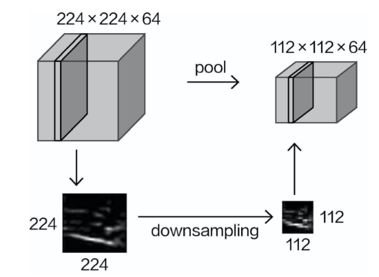
常用池化方法有最大池化和平均池化。

Common pooling methods include Max Pooling and Average Pooling.

最大池化的原理很简单，首先在输入特征图中选择各个区域，然后“计 算”其特征值，这里并没有像卷积层那样有实际的权重参数进行计算，而是直接选择最大的数值即可。

The principle of Max Pooling is very simple. First, select various regions in the input feature map, and then "compute" their feature values. Unlike the convolution layer, where actual weight parameters are involved in the calculation, here you simply choose the maximum value.

平均池化的基本原理也是一样，只不过在计算过程中，要计算区域的平均值，而不是直接选择最大值。

The basic principle of Average Pooling is the same, except that during the calculation, you compute the average value of the region instead of selecting the maximum value.

那么，是不是平均池化效果更好呢?并不是这样，现阶段使用的基本都是最大池化，感觉它与自然界中的优胜劣汰法则差不多，只会把最合适的保留下来，在神经网络中也是如此，需要最突出的特征。

So, does this mean that Average Pooling performs better? Not necessarily. Currently, Max Pooling is predominantly used. It seems to align with the "survival of the fittest" principle found in nature, where only the most suitable features are retained. Similarly, in neural networks, the most prominent features are needed.

卷积神经网络整体架构

Overall Architecture of a Convolutional Neural Network

卷积网络中可以调节的参数还有很多，网络结构肯定千变万化，那么，做实验时，是不是需要把所有可能都考虑进去呢?通常并不需要做这些基础实验，用前人实验好的经典网络结构是最省时省力的。所谓经典就是在各项竞赛和实际任务中，总结出来比较实用而且通用性很强的网络结构。

There are many adjustable parameters in a convolutional network, and the network structures can vary widely. So, when conducting experiments, do we need to consider every possible configuration? Usually, this is not necessary. Using classic network structures, which have been well-tested in previous experiments, is the most time-efficient and reliable approach. These classic structures are derived from various competitions and real-world tasks, and they have proven to be both practical and versatile.

在了解经典之前，还要知道基本的卷积神经网络模型，这里给大家先来总结一下。一个完整的卷积神经网络，首先对输入数据进行特征提取，然后完成分类任务。通常卷积 操作后，都会对其结果加入非线性变换，例如使用ReLU函数。池化操作与卷积操作是搭配来的，可以发 现卷积神经网络中经常伴随着一些规律出现，例如2次卷积后进行1次池化操作。最终还需将网络得到的 特征图结果使用全连接层进行整合，并完成分类任务，最后一步的前提是，要把特征图转换成特征向 量，因为卷积网络得到的特征图是一个三维的、立体的，而全连接层是使用权重参数矩阵计算的，也就 是全连接层的输入必须是特征向量，需要转换一下。

Before learning about the classic models, it's essential to understand the basic convolutional neural network model, which is summarized here. A complete convolutional neural network (CNN) first performs feature extraction on the input data and then completes a classification task. After each convolution operation, it's common to apply a non-linear transformation, such as using the ReLU function. Pooling operations often follow convolution operations, and a common pattern seen in CNNs is performing two convolution operations, followed by one pooling operation.

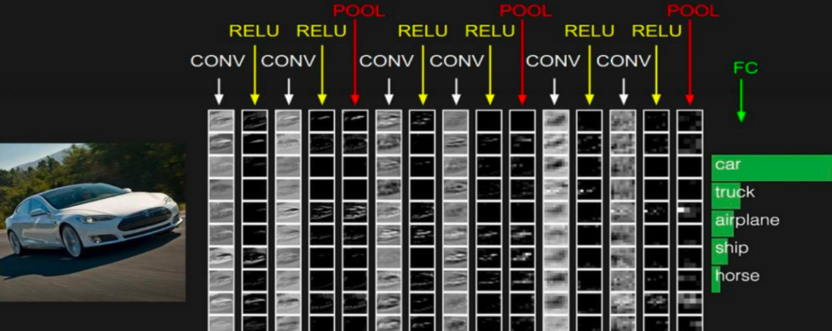
卷积神经网络的核心就是得到的特征图，如图所示，特征图的大小和个数始终在发生变化，通常卷积操作要得到更多的特征图来满足任务需求，而池化操作要进行压缩来降低特征图规模(池化时特征图个数不变)。最后再使用全连接层总结好全部特征，在这之前还需对特征图进行转换操作，可以当 作是一个把长方体的特征拉长成一维特征的过程。

Finally, the resulting feature maps from the network need to be integrated using a fully connected layer to complete the classification task. However, for this last step, the feature maps must first be converted into feature vectors, because the feature maps produced by the convolutional network are three-dimensional, while fully connected layers perform calculations using a weight matrix. Therefore, the input to the fully connected layer must be a feature vector, necessitating this conversion.

常见的卷积神经网络有：

Common Convolutional Neural Networks:

AlexNet网络：选择偏大的卷积核，提取的特征肯定不够细致，网络层数太少，提取不够细腻，估计还是硬件设备计算性能所限。

AlexNet: AlexNet uses relatively large convolutional kernels, meaning the extracted features may not be very detailed. The network has too few layers, so the extracted features are not fine enough. This is likely due to the limited computational performance of hardware at that time.

VGG网络网络：由于VGG网络层数比较多，有好几种版本，其使用价 值至今还在延续，所以很值得学习。

VGG Network: Since the VGG network has many layers and several versions, its practical value continues to this day, making it well worth studying.

VGG网络有一个特性，所有卷积层的卷积核大小都是3×3，可以用较小的卷积核来提取特征，并且加入更多的卷积层。这样做有什么好处呢?还需要解释一个知识 点—感受野，它表示特征图能代表原始图像的大小，也就是特征图能感受到原始输入多大的区域。现在要求它的感受野，也就是它能看到原始输出多大的区域。

One characteristic of the VGG network is that all convolutional layers use kernels of size 3×3, allowing for feature extraction with smaller kernels and the addition of more convolutional layers. What is the benefit of this? To explain, we need to introduce the concept of the receptive field, which refers to the size of the original image that a feature map can represent—that is, the area of the original input that the feature map can "sense."

倒着来推，它能看到第一个特征图3×3 的区域(因为卷积核都是3×3的)，而第一个特征图3×3的区域能看到原始输入5×5的区域，此时就说当前的感受野是5×5。通常都是希望感受野越大越好，这样每一个特征图上的点利用原始数据的信息就更多

To calculate the receptive field, you can work backwards. The first feature map is influenced by a 3×3 region (since the convolutional kernels are all 3×3), and this 3×3 region can "see" a 5×5 area of the original input. In this case, we say the current receptive field is 5×5. Generally, we want the receptive field to be as large as possible so that each point in the feature map utilizes as much information from the original data as possible.

ResNet网络：其核心思想是每个附加层都应该更容易地包含原始函数作为其元素之一。

ResNet Network：The core idea of ResNet is that each additional layer should more easily include the original function as one of its components.

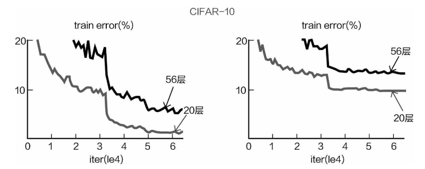
通过之前的对比，大家发现深度网络的效果更好，那么为什么不让网络再深一点呢?100层、1000层 可不可以呢?理论上是可行的，但是先来看看之前遇到的问题。如图所示，如果沿用VGG的思想将网络继续堆叠得到的效果并不好，深层的网络(如56层)无 论是在训练集还是在测试集上的效果都不理想，那么所谓的深度学习是不是到此为止呢?在解决问题的 过程中，又一神作诞生了——深度残差网络。

From previous comparisons, we can see that deeper networks tend to perform better. So, why not make the network even deeper? What about 100 layers, or even 1,000 layers? In theory, this is possible, but first, let’s look at the problems encountered before. As shown in the diagram, if we continue stacking layers following the VGG approach, the results do not improve. Deep networks (such as 56-layer networks) perform poorly on both the training set and the test set. Does this mean that the concept of deep learning has reached its limit? Fortunately, another breakthrough came along to solve this issue—the Deep Residual Network (ResNet).

其基本思想就是，因网络层数继续增多，导致结果下降，其原因肯定是网络中有些层学习得不好。 但是，在继续堆叠过程中，可能有些层学习得还不错，还可以被利用。

The basic idea is that, as the number of layers increases, performance deteriorates. This is likely because some layers in the network do not learn well. However, during the stacking process, some layers may still learn useful representations and can be further utilized.

图为ResNet网络叠加方法。如果这样设计网络结构，相当于输入x(可以当作特征图)在进行卷 积操作的时候分两条路走:一条路中，x什么都不做，直接拿过来得到当前输出结果;另一条路中，x需 要通过两次卷积操作，以得到其特征图结果。再把这两次的结果加到一起，这就相当于让网络自己判断 哪一种方式更好，如果通过卷积操作后，效果反而下降，那就直接用原始的输入x;如果效果提升，就把 卷积后的结果加进来。

In this figure, the ResNet stacking method is illustrated. In this structure, the input x (which can be thought of as a feature map) follows two paths during the convolution operation: one path where x is left unchanged and directly used to obtain the current output, and another path where x undergoes two convolution operations to generate a feature map. The results from both paths are then added together. This effectively allows the network to decide which method is better: if the result after convolution degrades performance, the network will simply use the original input x; if the results improve, the convolution output is added to the input.

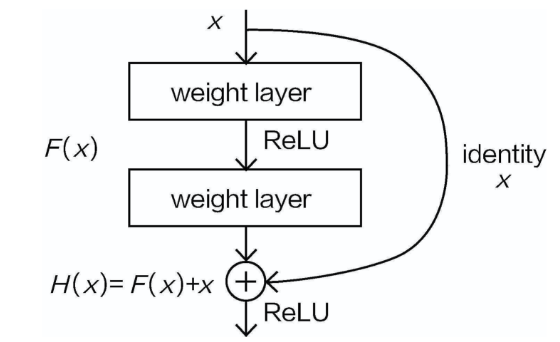
这就解决了之前提出的问题，深度网络模型可能会导致整体效果还不如之前浅层的。按照残差网络 的设计，继续堆叠网络层数并不会使得效果下降，最差也是跟之前一样。如图19-29所示，图19-29(a)就是用类似VGG的方法堆叠更深层网络模型，层数越多，效果反而越差。图19-29(b)是ResNet，它完美地解决了深度网络所遇到的问题。

This approach solves the previous issue where deeper networks sometimes performed worse than shallower ones. According to the design of the residual network, stacking more layers will not degrade performance—in the worst case, it will remain the same as before. As shown in Figures 19-29, Figure 19-29(a) shows how simply stacking deeper layers using a VGG-like approach leads to worse performance with more layers. Figure 19-29(b) shows ResNet, which perfectly solves the problems associated with very deep networks.

图片分类代码示例 

Image Classification Code Example

学习了卷积原理之后，还要用TensorFlow实际把任务做出来。依旧是Mnist数据集，只不过这回用卷积神经网络来进行分类任务，不同之处是输入数据的处理:

After learning the principles of convolution, it's time to implement the task using TensorFlow. We will once again use the MNIST dataset, but this time we'll use a convolutional neural network for the classification task. The difference lies in how the input data is processed:

构建模型

Building the Model

import tensorflow as tf
import numpy as np
import os
import matplotlib.pyplot as plt

# 使用Sequential API定义模型
model = tf.keras.models.Sequential()

# 第一个卷积层：32个3x3卷积核，激活函数ReLU，采用SAME padding
model.add(tf.keras.layers.Conv2D(32, (3, 3), activation='relu', padding='same', input_shape=(28, 28, 1)))

# 第二个卷积层：64个3x3卷积核，激活函数ReLU，SAME padding
model.add(tf.keras.layers.Conv2D(64, (3, 3), activation='relu', padding='same'))

# 最大池化层：2x2池化窗口
model.add(tf.keras.layers.MaxPooling2D(pool_size=(2, 2)))

# Dropout层：丢弃50%的神经元
model.add(tf.keras.layers.Dropout(0.25))

# 将多维特征图拉平成一维
model.add(tf.keras.layers.Flatten())

# 全连接层：128个神经元，激活函数ReLU
model.add(tf.keras.layers.Dense(128, activation='relu'))

# Dropout层：丢弃50%的神经元
model.add(tf.keras.layers.Dropout(0.5))

# 输出层：10个神经元（对应10个类别），使用softmax激活函数
model.add(tf.keras.layers.Dense(10, activation='softmax'))

编译模型并训练

Compile the Model and Train

# 编译模型，指定损失函数、优化器和评估指标
model.compile(loss='categorical_crossentropy',
              optimizer=tf.keras.optimizers.Adam(),
              metrics=['accuracy'])
              
# 设置超参数
batch_size = 50
epochs = 10

# 训练模型
history = model.fit(x_train, y_train,
                    batch_size=batch_size,
                    epochs=epochs,
                    validation_data=(x_test, y_test),
                    verbose=1)

评估结果

Evaluate Results

# 在测试集上评估模型
test_loss, test_acc = model.evaluate(x_test, y_test, verbose=2)
print(f'\n测试集上的准确率: {test_acc:.4f}')

# 6. 进行所有测试集的预测
predictions = model.predict(x_test)

# 将预测结果转换为类别索引
predicted_labels = np.argmax(predictions, axis=1)

# 7. 找到预测错误的样本
# 将真实标签从 one-hot 编码转换为类别索引
true_labels = np.argmax(y_test, axis=1)
# 找到预测错误的样本索引
incorrect_indices = np.where(predicted_labels != true_labels)[0]
# 打印前5个预测错误的样本
print(f"找到{len(incorrect_indices)}个预测错误的样本。")

# 8. 可视化前几个预测错误的样本
num_to_display = 5  # 要展示的错误样本数量
plt.figure(figsize=(10, 5))
for i, idx in enumerate(incorrect_indices[:num_to_display]):
    plt.subplot(1, num_to_display, i + 1)
    plt.imshow(x_test[idx].reshape(28, 28), cmap='gray')
    plt.title(f"True: {true_labels[idx]}, Pred: {predicted_labels[idx]}")
    plt.axis('off')
plt.tight_layout()
plt.show()

相比之前神经网络代码运行结果的200+识别错误，卷积神经网络虽然耗时多了一些，但准确率高很多

Compared to the 200+ recognition errors in the previous neural network code, the convolutional neural network takes more time but achieves significantly higher accuracy.